Rhino Strategy Family: From Broken-Wing Butterfly to Genetic Optimization

The Rhino Options Strategy is a conservative, broken‑wing butterfly income trade with an upside hedge. Rhino is not just a simple trade; it’s a whole family of related strategies that have evolved over nearly a decade in response to changing market conditions.

Monthly, Giant, and Baby Rhino variants coexist alongside variants from other developers like the White Rhino by Randy Schwartzenburg. Several modern income trades share similar DNA: Amy Meissner’s A14, the BWB‑Cal trades from Ron Bertino, and more recent public trades such as Time Flies Spread and Flyagonal.

They all blend a put‑side income structure with a calendar or diagonal hedge. Whether they were directly inspired by the Rhino or evolved in parallel, they live in the same design space.

In this article we will show how Rhino has evolved, share our personal experience with related strategies, and we use a Genetic Algorithm to provide a variant that works well in recent market conditions.

This will be a long one, settle in like you accidentally picked the director’s cut.

TL;DR: Performance at a glance

• Original conservative SPX Rhino (2018–2025): Sharpe 1.12, CAGR 3.15%, MaxDD −2.81%
• GeneticRhino-25Q4 (IS 2022–2025 / OOS 2018–2022):
  • IS Sharpe 2.31, CAGR 13.1%, MaxDD −4.2%, Deflated Sharpe: 1.15
  • OOS Sharpe 2.2, CAGR 9.21%, MaxDD −6.74%
  • Same design space (BWB + call hedge), simplified rules, GA + DSR to control overfitting.

---

Overview

The Rhino Options Strategy was developed by Brian Larson and published at Capital Discussions (now Aeromir) in 2015. After the initial publication, Bruno Voisin played a major role in the strategy development and has been steadily refining the trade ever since.

At its core, the trade combines:

• An out‑of‑the‑money put broken‑wing butterfly (BWB)
• An upside hedge — typically call calendars

Rhino Shape

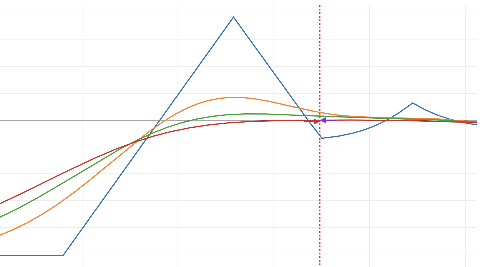
The risk graph resembles a Rhino’s head: the BWB and the upside hedge form two horns, with a broad, relatively flat T+0 between them.

Trade characteristics:

• Flat or slightly negative delta over a wide range
• Low gamma
• Positive theta that doesn’t require hyper‑active management

The Rhino family directly shaped MesoSim's approach to leg selection and adjustments, therefore it is ideal to showcase MesoSim's capabilities.

Foreword

Most Rhino variants are discretionary to some degree. In such setups, the delta limits, scaling decisions, and hedge choices are guidelines, rather than a strict algorithm.

These are often choices of the developer. To quote Bruno:

I would never use specific mechanical rules, simple or sophisticated, and instead chose meta parameters in the form of risk management ratios combining margin and Greeks.

While we respect Bruno's opinion, we believe that clear rules are essential for trading, at least when it comes to strategies we trade. This disparity is common in the trading world: traders are frequently opinionated and there is no single "correct" way to trade.

When recreating these trades in MesoSim, we aimed to:

• Respect the spirit of each author’s intent
• Acknowledge that any exact rule set we encode will inevitably reflect some of our choices.

To keep things honest, we share backtests based on the rules available at the time of development.

The Rhino’s evolution is a case study in that principle.

History

If you are interested in the detailed evolution of the Rhino strategy, please click the Rhino Development History below. It contains a summary from all the presentations from Brian and Bruno, highlighting the key changes over time. We included the presentation links for reference.

Rhino Development History

2014-2017: Early Rhino

The early Rhino, as documented in the Original Video and Bruno's 2016 and 2017 deck, is a fixed‑distance RUT BWB with clear delta triggers and a profit target ladder.

Core features:

• RUT focus – Five 50/40 put BWBs with upper longs 10–15 points ITM (later 0.5–1% ITM).
• SPX variant – Three 80/60 put BWBs (later 100/75 and 75/50 wings) with similar upper‑long bias.
• Entry – Around 77 DTE on a down day if possible, to launch with a flat T+0 line and conservative downside coverage of roughly 5–7%. $25k planned capital per cycle.
• Adjustment logic –
  • Negative delta beyond −25 (half) / −50 (full) → add call calendars, put verticals or condors, occasionally roll back BWBs.
  • Positive delta beyond +25 → remove or roll hedges/BWBs to flatten.
• Exit – :
  • The profit ladder (10/8/6/4%)
  • Exiting before gamma “gets hard to handle” (generally before ~21 DTE)

The trade assumes a fairly “normal” volatility regime. Fixed strikes and ATM entries mean:

• In very low vol, the tent is narrow and profits harder to reach.
• In very high vol, more capital sits near the money, and large moves require heavier hedging.

2017–2019: from trade to trade family

By 2017–2018, Bruno emphasized that the real Rhino is less a single trade and more a family of BWBs run as a capital‑allocation process.

Two ideas arrive here:

1. Trade phases

   From the 2018 decks (deck 1, deck 2, deck 3 and deck 4):

   • Take‑off (Growth) – From entry (~77 DTE) down to roughly 49–56 DTE. Build up to full size, preferably on down days.
   • Cruise (Maturity) – From there down to around 28–35 DTE. Hold capital constant, focus on Greeks.
   • Descent (Getting Old) – Roughly 35–21 DTE, later tightening to 28–14 DTE. Protect profits, peel off, avoid loading gamma.

   Each capital reallocation step (scale‑in, peel‑off, roll) is a chance to rebalance delta and gamma, with delta triggers becoming a “measure of last resort” rather than the primary decision driver.

2. Horizontal layering & the Rhino family

   The 2019 Rhino Strategy formalises three related trades:

   • Monthly Rhino – The original 77→14 DTE cycle.
   • Giant Rhino – Longer‑dated version (~100–120 DTE into ~35 DTE).
   • Baby Rhino – Weekly 14→7 DTE short‑duration BWB, essentially a theta game on a short fly.

   Overlapping these cycles at different expirations introduces horizontal layering — smoothing P&L and turning the Rhino into a small BWB portfolio rather than a single isolated position.

Delta triggers also get sharpened:

• Downside: trigger if delta < −5 per BWB inside the tent.
• Upside: trigger when delta > 5 per BWB (roughly 25 per BWB at full size), and when the lowest shorts are being passed.

2020-2022: Volatility-adaptive structures

The Evolving Rhino presentation emphesizes that the ruling principle of the trade:

“A flattish Delta over the largest possible range.”

Everything else — entry, wings, hedges, capital — is adjusted to serve that principle in a volatile, post‑2018 market.

Key changes from that presentation and the 2022 high‑vol update:

1. OTM entries & larger wings in high vol

   • ATM entries in high vol tend to start with positive delta and a very pressurised T+0.
   • Solution: move the BWB further OTM and increase wing sizes when VIX is high.

   “Major Changes (1)” section introduces simple rules of thumb for SPX:

   • Low vol (VIX ≲ 12.5): wings ≈ 75/50
   • Normal vol (≈12.5–19.5): wings ≈ 100/75
   • High vol (VIX ≳ 19.5): wings ≈ 125/100

   The PDS (debit) wing is weaker on an OTM Rhino, but the trade gains robustness in volatile markets and is less sensitive to “vol pops.”

2. Phase‑based capital management

   • Take‑off: build to planned capital by about 49 DTE.
   • Cruise: keep capital stable 49→28 DTE.
   • Descent: gradually cut exposure 28→10–14 DTE and either exit or leave at most ¼ of planned capital in the old cycle.

3. Risk metrics: MtE & VaR

   Rather than managing only by per‑trade delta, Bruno introduces:

   • Margin‑to‑expiration (MtE) bands (or similar VaR‑style limits) across all open cycles:
     • Conservative: 35% with occasional peaks to 45%
     • Balanced: 50% with peaks to 60%
     • Aggressive: 65% with peaks to 70%

   Delta triggers remain, but capital and margin become the primary risk knobs.

4. Hedging style

   • Upside – Narrow 30‑delta call calendars placed above strong resistance levels act as “speedbumps” in bullish high‑vol regimes.
   • Downside – Layered convexity:
     • Inner put debit spreads, outer put credit spreads (PDS/PCS).
     • Occasional put calendar below the lowest shorts, particularly as part of a “roll in one go” crash response.

5. Profit expectations

   In this high‑vol, conservative variant Bruno explicitly sets:

   • Profit target: around 2% of planned capital per cycle
   • Exit at ~14 DTE or reduce exposure to ≤¼ planned capital

The modern conservative Rhino is therefore:

• Still recognisably the same trade
• Less about rigid delta numbers, more about MtE bands, overlapping cycles, and a flattish delta shape across regimes

2023: Flexibility to adapt to lower vol & 0DTE effects

The 2023 “An Overdue Rhino Update” revisits the strategy in the context of today’s market: lower headline volatility but heavy 0-DTE activity, Interest Rate changes and fast‑flipping regimes.

Key messages:

1. Environment: lower vol is not automatically safer

   • Volatility regimes are changing rapidly; SPX and VIX still mean‑revert against each other, but their correlation can be unstable.
   • Interest rates have moved but remain moderate; for options traders, the more important changes are in equity risk appetite and FX correlations.
   • A huge share of CBOE volume is now 0DTE. On some days these flows approach 50% of volume, concentrating dealer gamma and creating strong intraday “attractors.”

   The takeaway: “Lower volatility = higher risk” for a slow income trade that sells options across weeks, because short‑dated order flow can whip prices through your tent.

2. Market reading: a “delta‑neutral” trade is not market‑neutral

   Bruno doubles down on basic market reading:

   • Use simple chart levels: support/resistance, fibs, basic patterns.
   • Track key drivers like the big tech stocks and correlated indices (NDX, DJI).
   • Watch dealer gamma and vanna (GEX & VEX) to understand where dealers are likely to push or defend prices.

3. What has changed: more flexibility

   The “What has changed” slide highlights flexibility and tool choice in lower‑vol conditions:

   • The “typical” BWB (on 25‑point strikes in his book) can sometimes be replaced with a split‑strike BWB to better fit local skew.
   • Call calendars can be substituted with call diagonals where the goal is to “go with the flow” — participating in bullish moves while keeping vega exposure smaller than with horizontal spreads.
   • When the trader admits to being “totally lost” about short‑term direction, Bruno suggests falling back on a reasonable delta/vega ratio, roughly similar to the balanced profile used in the cruise phase.

   In other words, the modern Rhino toolkit is broader: calendars, diagonals, split‑strike BWBs, balanced flies all live under the same philosophy.

Rhino in MesoSim

Many variants - public and proprietary - of the Rhino trade exist as MesoSim Strategy Definitions, and we can’t cover them all here. We will try to capture the final version presented by Bruno in 2023, with some adjustments to match our personal beliefs and preferences.

Our preferences

There are, however, some aspects we have adjusted to match our personal beliefs and preferences:

• The market reading part (support / resistance, fibs, chart patterns) is excluded as we accept the thesis provided by David Aronson in his Evidence Based Technical Analysis book.
• The upside hedge (Call Calendar) side is added from the beginning of the trade.
• The structure is delta-neutral at initiation

We used ChatGPT for Strategy Development:

• GPT-5 Pro model with Extended Thinking time was used to obtain the trade rules. We provided the model with all the public presentations (available in the History section above), and asked it to summarise the latest rules of the trade.
• The MesoSim AI Agent was used to convert the rules into MesoSim Strategy Definition. The agent is a GPT-5 based assistant trained on MesoSim's documentation, strategies and blog posts.
• We reviewed the generated Strategy Definition and confirmed it is aligned with the public presentations. We needed to adjust the adjustment trigger delta and the Concurrency.MaxPositionsInFlight to match the trade plan.

The resulting Strategy Definition can be summarized as follows:

Underlying: SPX

Tenors: front month around ~77 DTE (window 56–84), back month ~107 DTE.

Core structure at entry (5 legs):

Parameter	VIX < 12.5	12.5 < VIX < 19.5	VIX > 19.5
BWB Upper Long OTM offset from ATM	15 pts	25 pts	35 pts
BWB Upper Long - Shorts width	75 pts	100 pts	125 pts
BWB Shorts - Lower Long width	50 pts	75 pts	100 pts
Calendar Shorts Delta	30 Δ	30 Δ	30 Δ
Calendar Longs Delta	30 Δ	30 Δ	30 Δ

Entry: Daily, 30 min before close, only on “very down day”: price < open < prior close. Concurrency allows up to 9 positions with 7-day entry spacing.

Adjustments: Daily, 30 min before close

• Phase 2 BWB: If the original’s DTE in [49,56] and only the 5 initial legs are open, add a second BWB (same VIX-mapped logic).
• Delta guards with calendars:
  • If pos_delta < −5 and no second calendar yet, add a second call calendar (front short ~30Δ, back long Δ ≈ |pos_delta|)
  • If pos_delta > 25, remove all calendar legs.
• Downside repair: If spot < BWB short strike, add a put debit spread (−1 at short_strike−10pts / +1 at short_strike−30pts ).
• De-risk late: If the extra BWB exists and the first BWB’s DTE ≤ 28, remove the second BWB set.

Exit: Daily, 30 min before close; profit target = $500, stop loss = $2,500 (both constants scaled from $25k base); OR exit if front BWB DTE ≤ 14

Fills, fees, margin: At mid (no slippage), $1.50/contract, PM-like margin

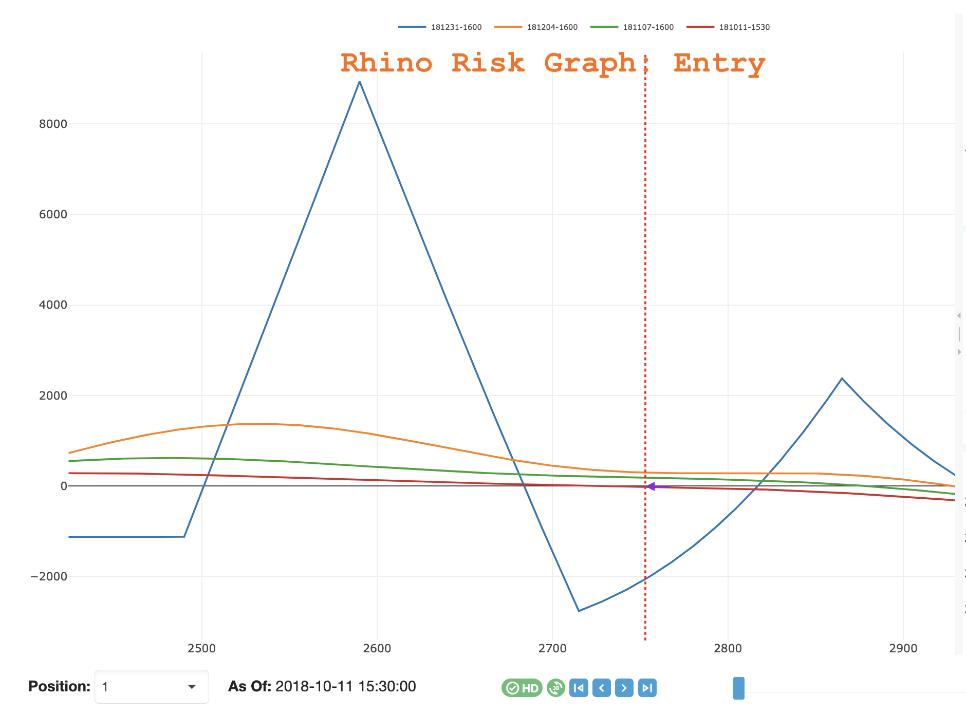
Risk Graphs

Here are the Risk Graphs at various stages:

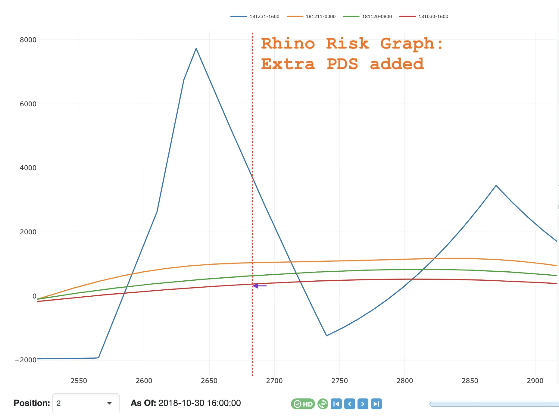
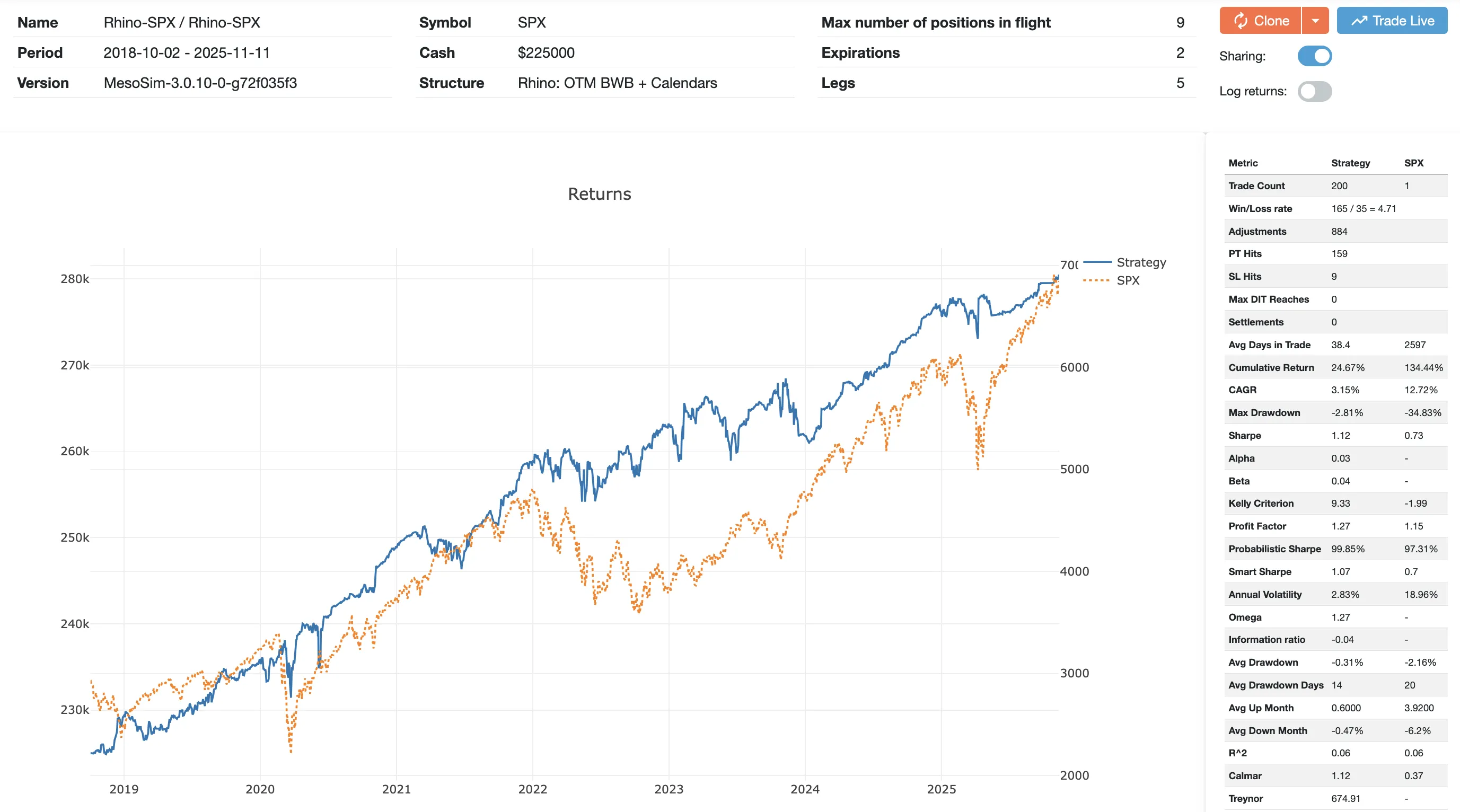
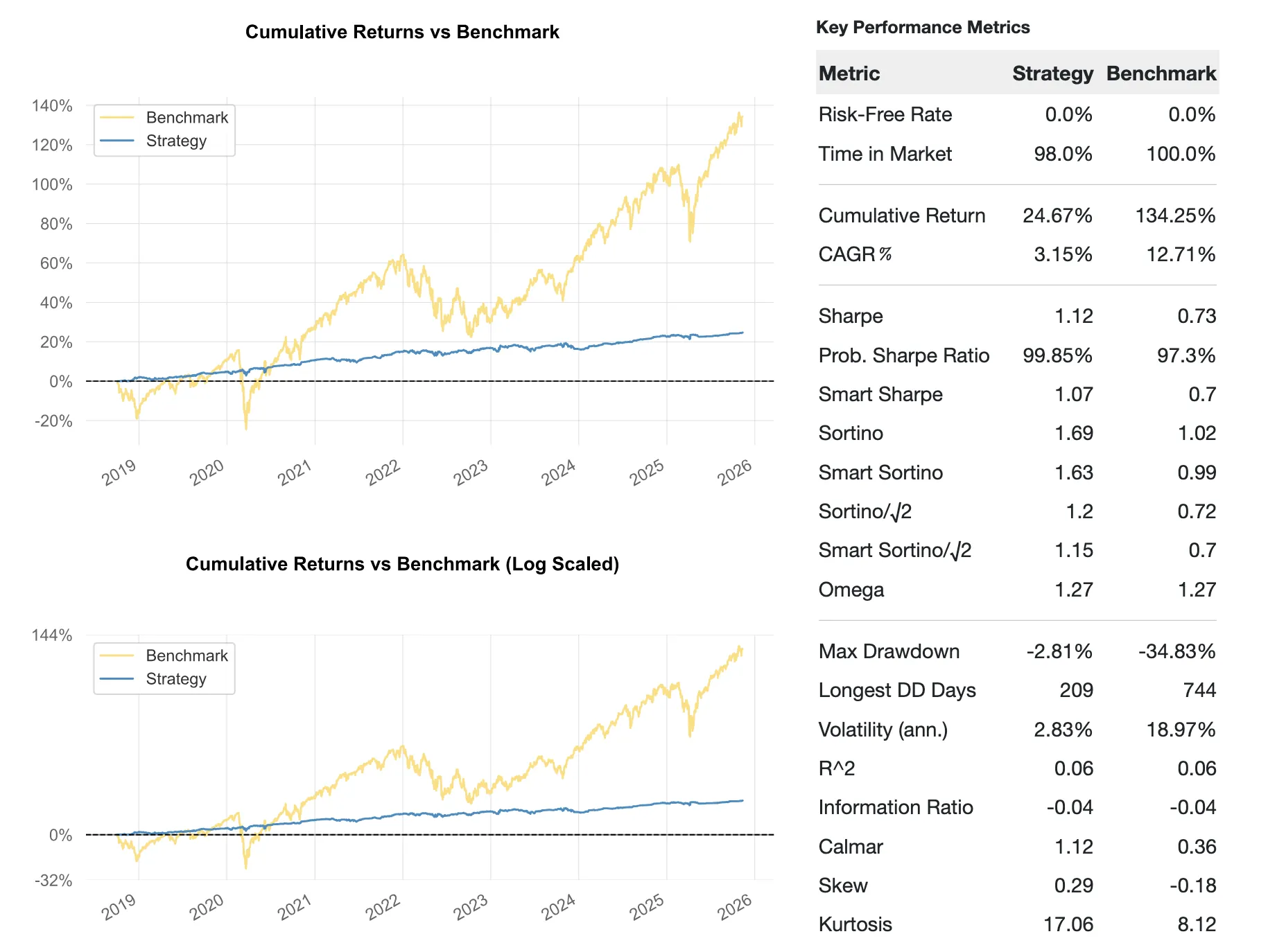
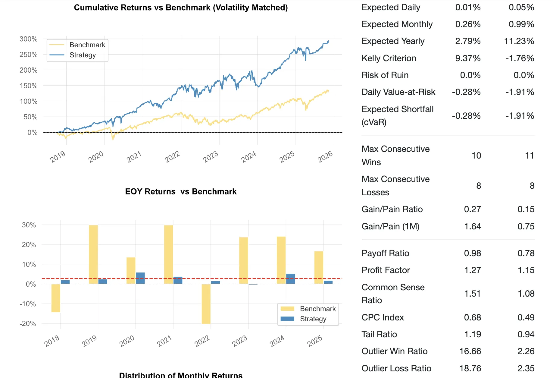
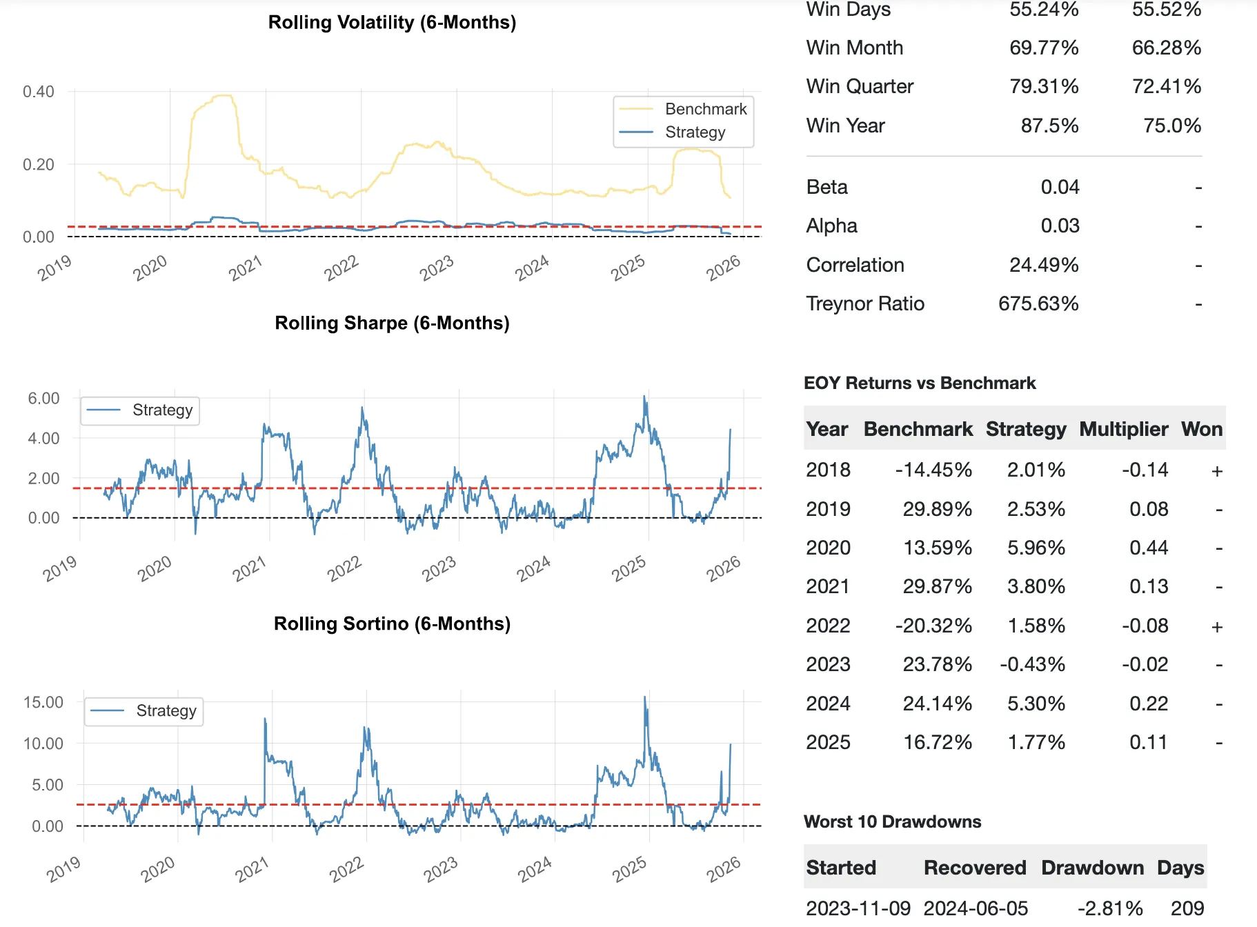
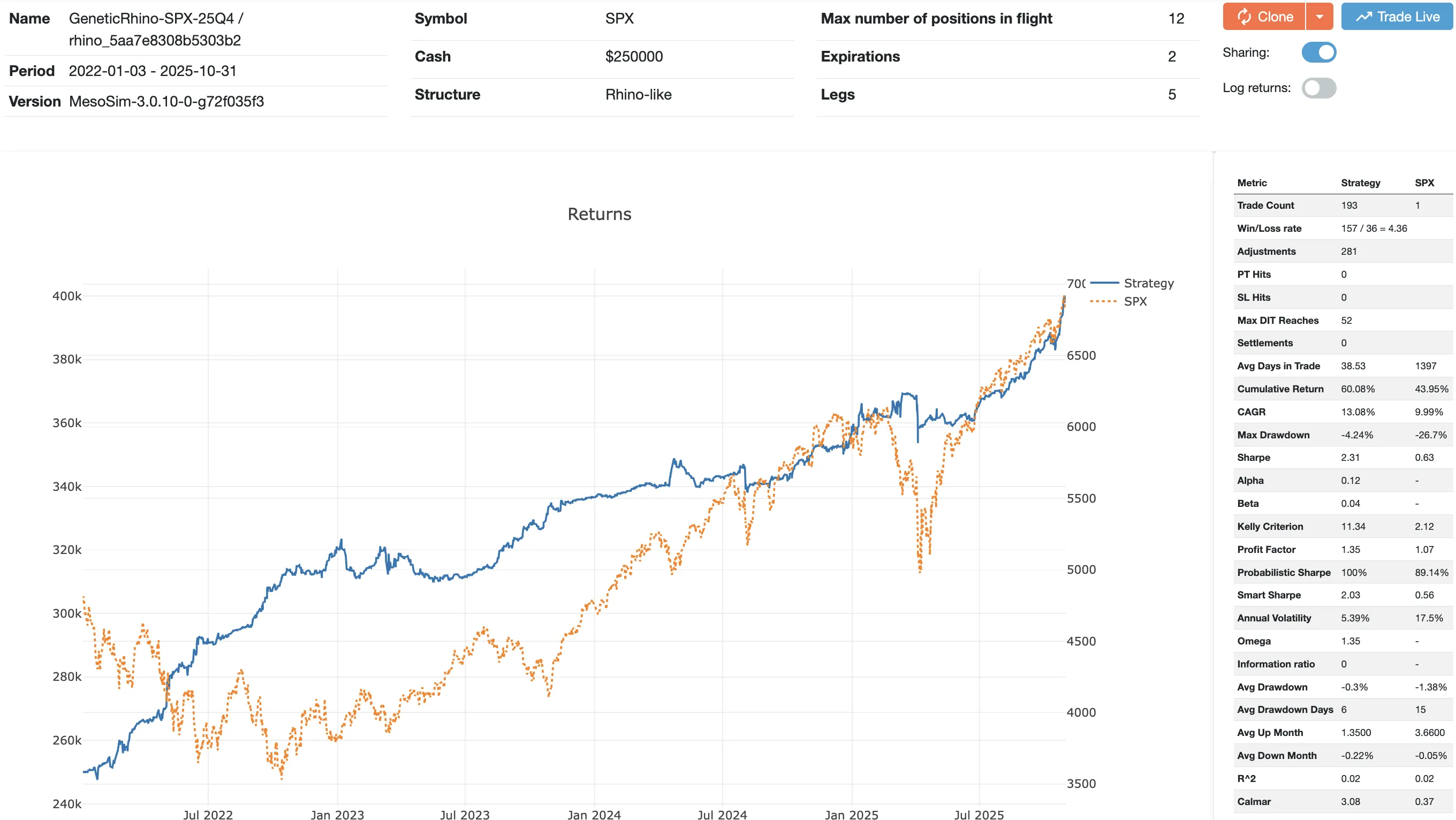
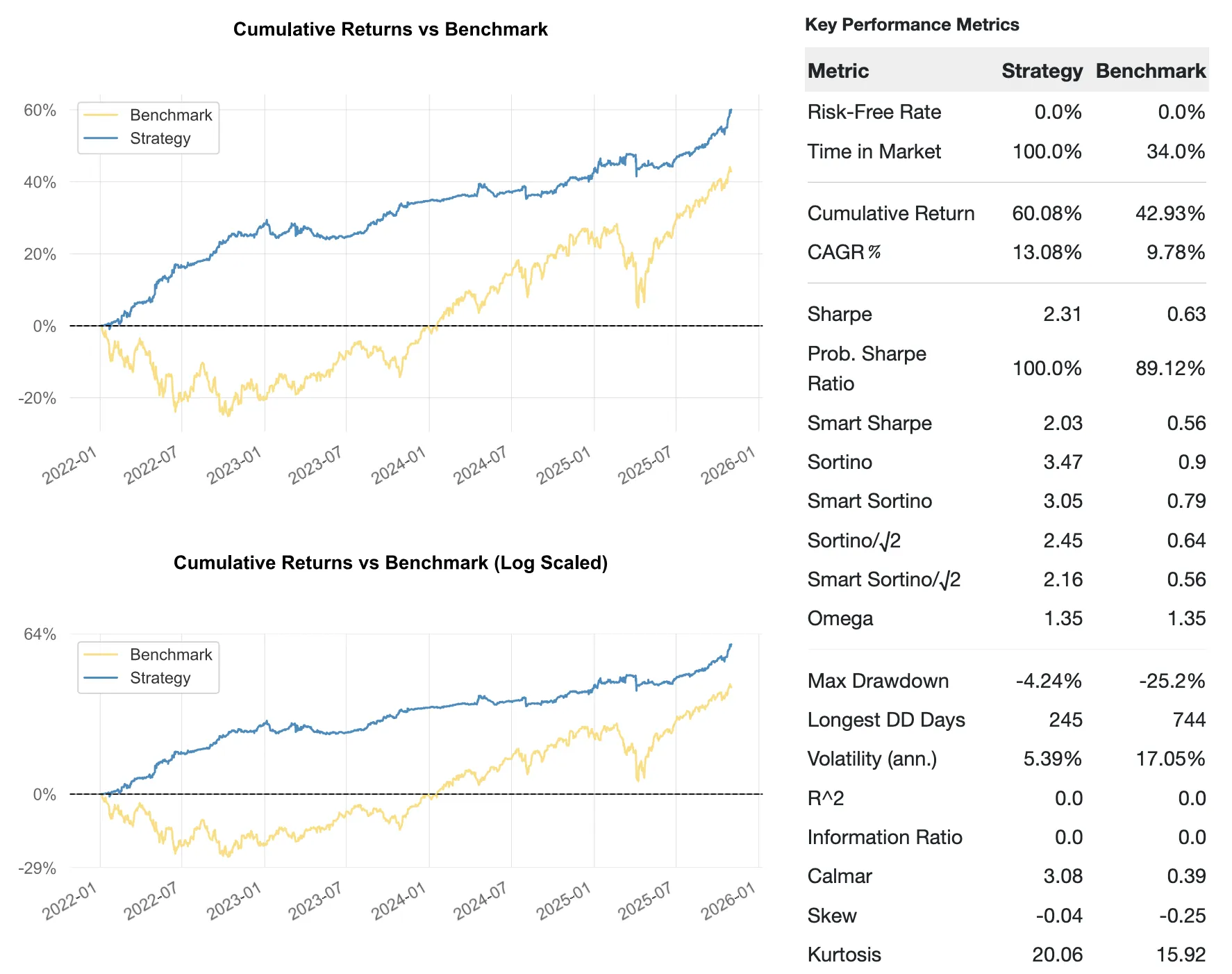
Backtest Summary

• MesoSim run: Rhino-SPX
• Backtest period: 2018-01-01 to 2025-11-11
• Sharpe Ratio: 1.12
• CAGR / Max Drawdown: 3.15% / -2.81%

tip

The above implementation is a fairly complex Strategy Definition, with multiple adjustments (structures added dynamically), scaling rules, and risk checks. If you need help understanding the Strategy Definition elements you can paste the Strategy Definition to the MesoSim AI agent and ask for explanations. You can start here: Explain the Rhino Strategy Definition

Other variants

A little detour to mention related trades we have first-hand experience with: A14 and BWB-Cal.

note

Because the A14 and BWB‑CD are proprietary trades, we won’t publish their MesoSim strategy definitions. We can provide them on request where the requester’s eligibility (e.g. active membership in the relevant service) can be verified.

A14 by Amy Meissner

The A14 Trade was developed by Amy Meissner and can be obtained (for a fee) from Aeromir. We got to know A14 before the Rhino and it influenced how MesoSim adjustments were designed.

Our live trading experience showed that the volatility of the strategy is beyond our comfort zone and we stopped trading it after a few cycles.

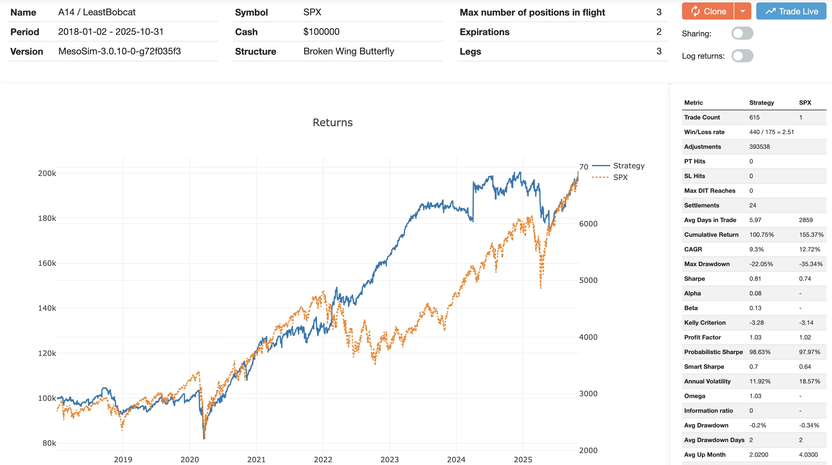
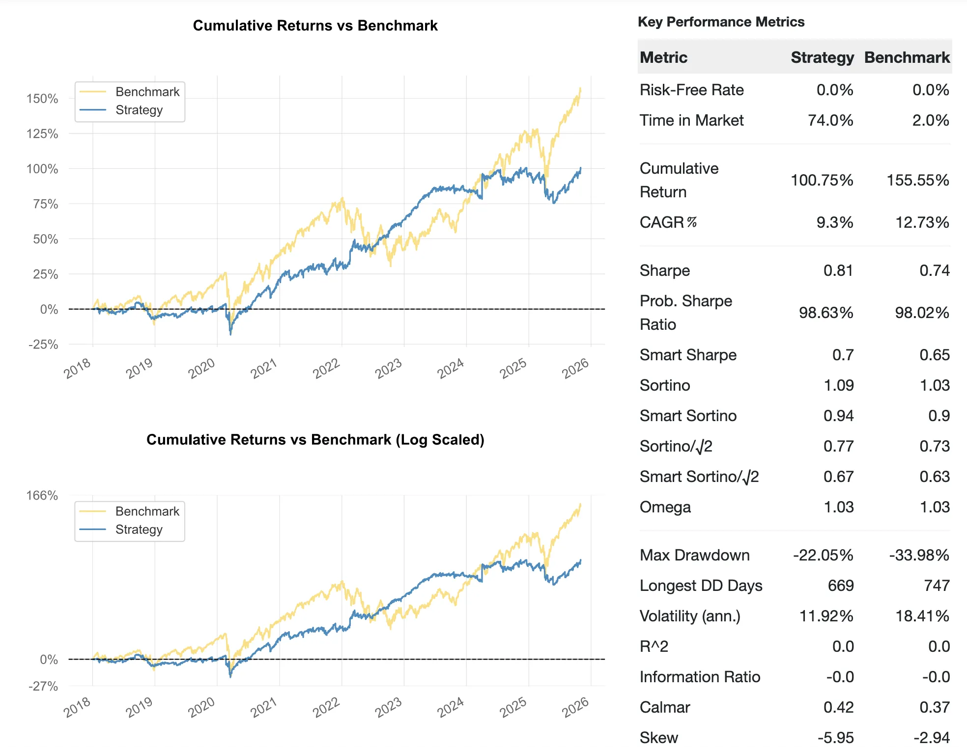
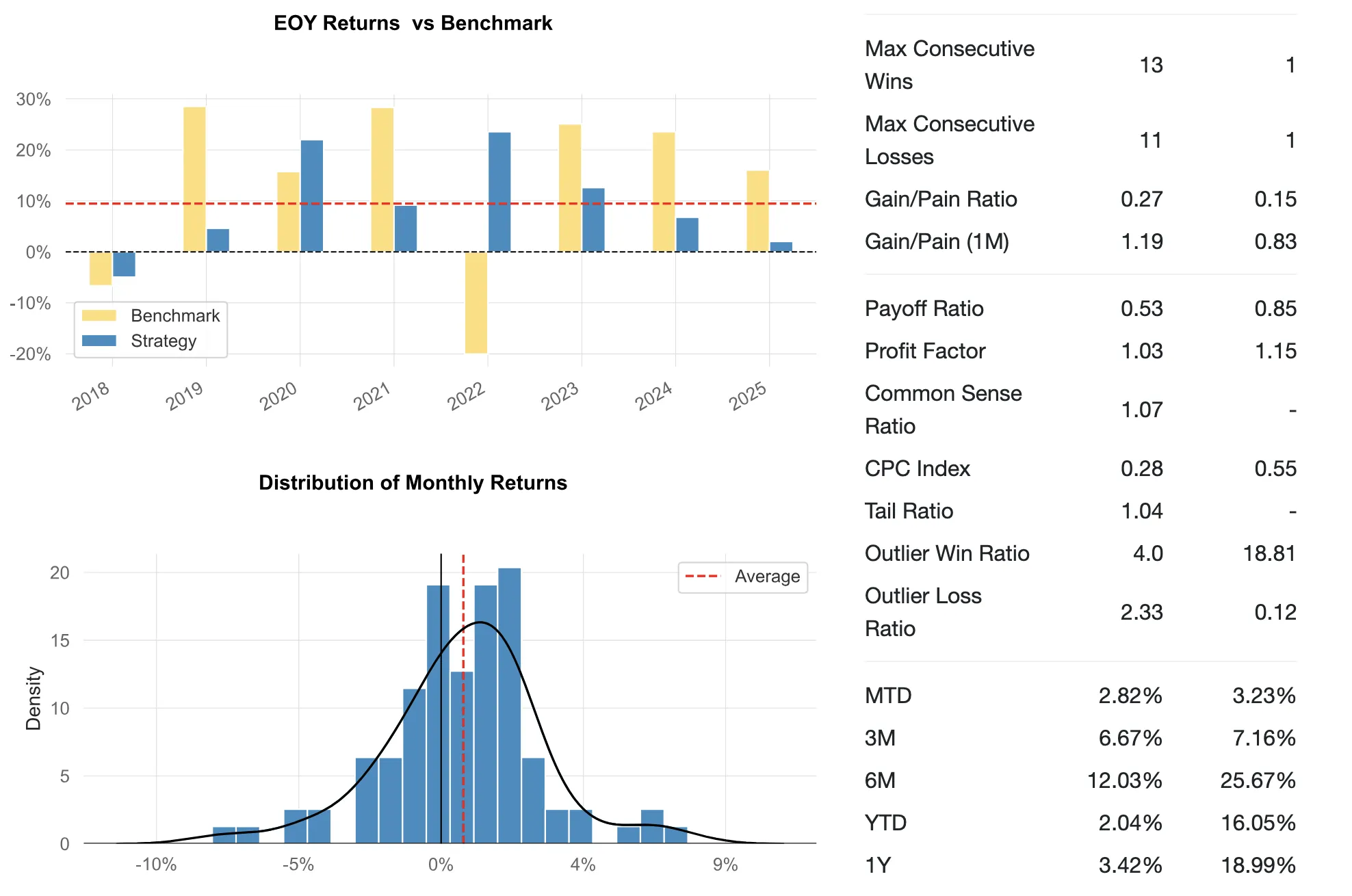
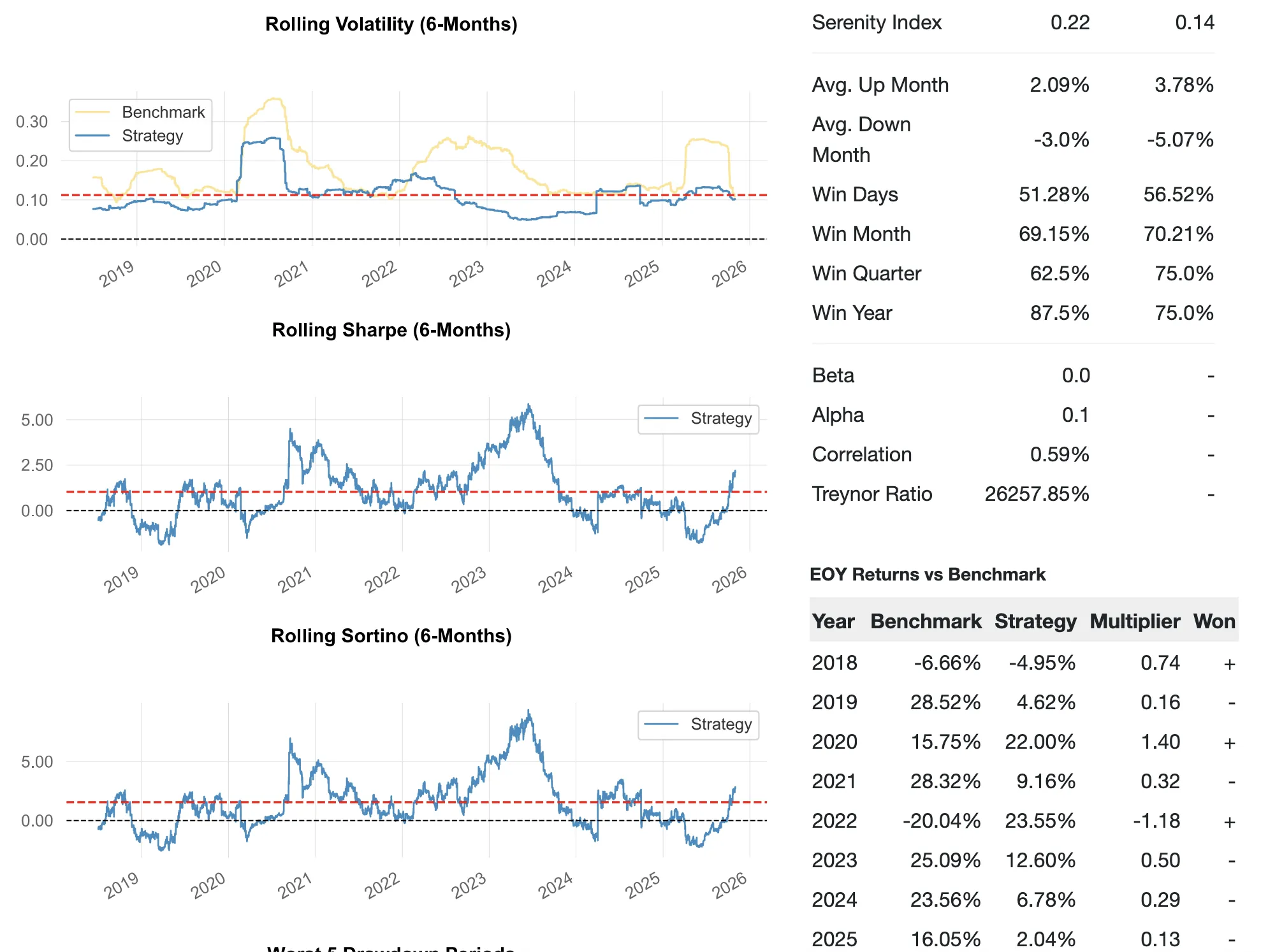
Backtest Summary

• Backtest period: 2018-01-01 to 2025-11-11
• Sharpe Ratio: 0.81
• CAGR / Max Drawdown: 9.3% / -22.05%

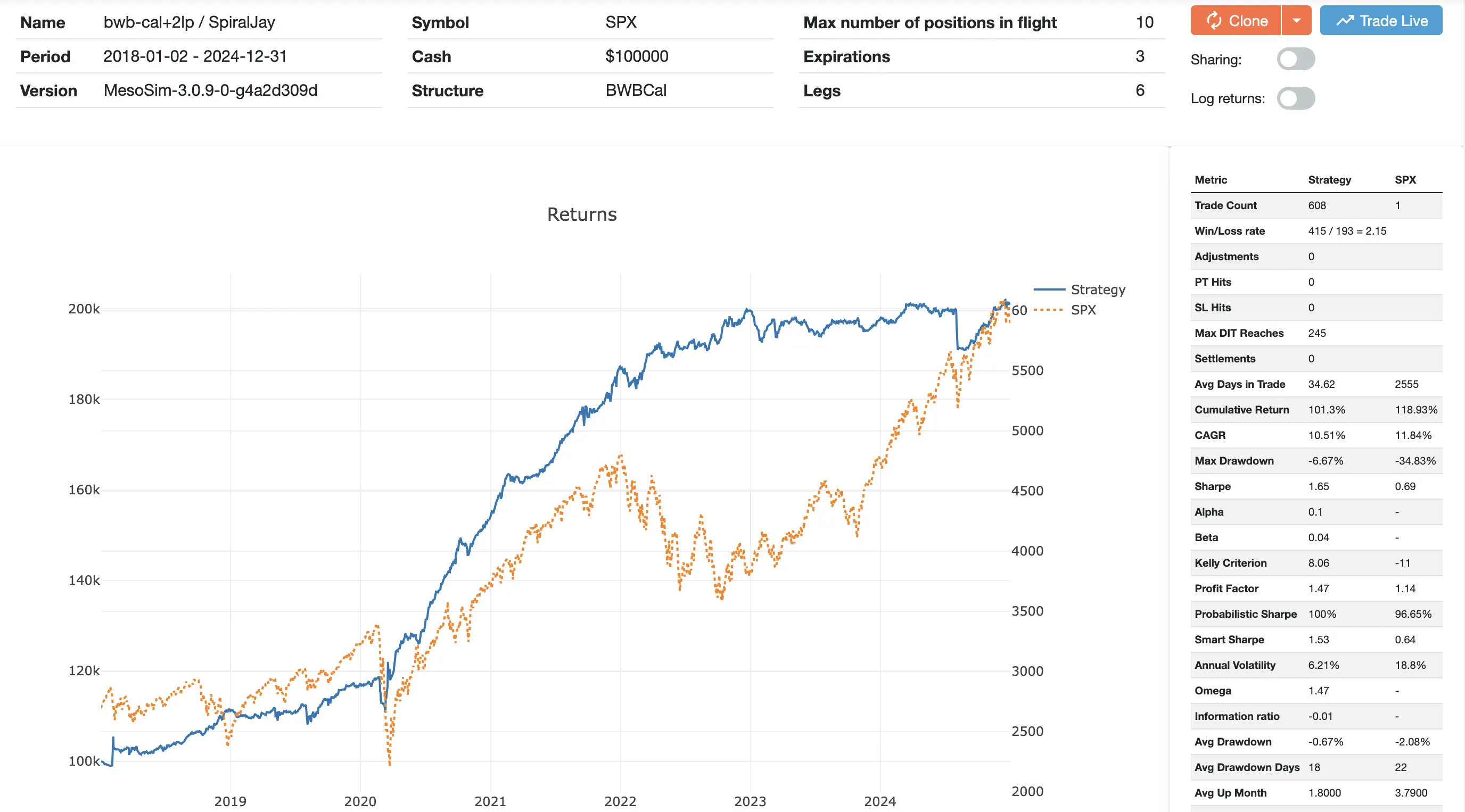
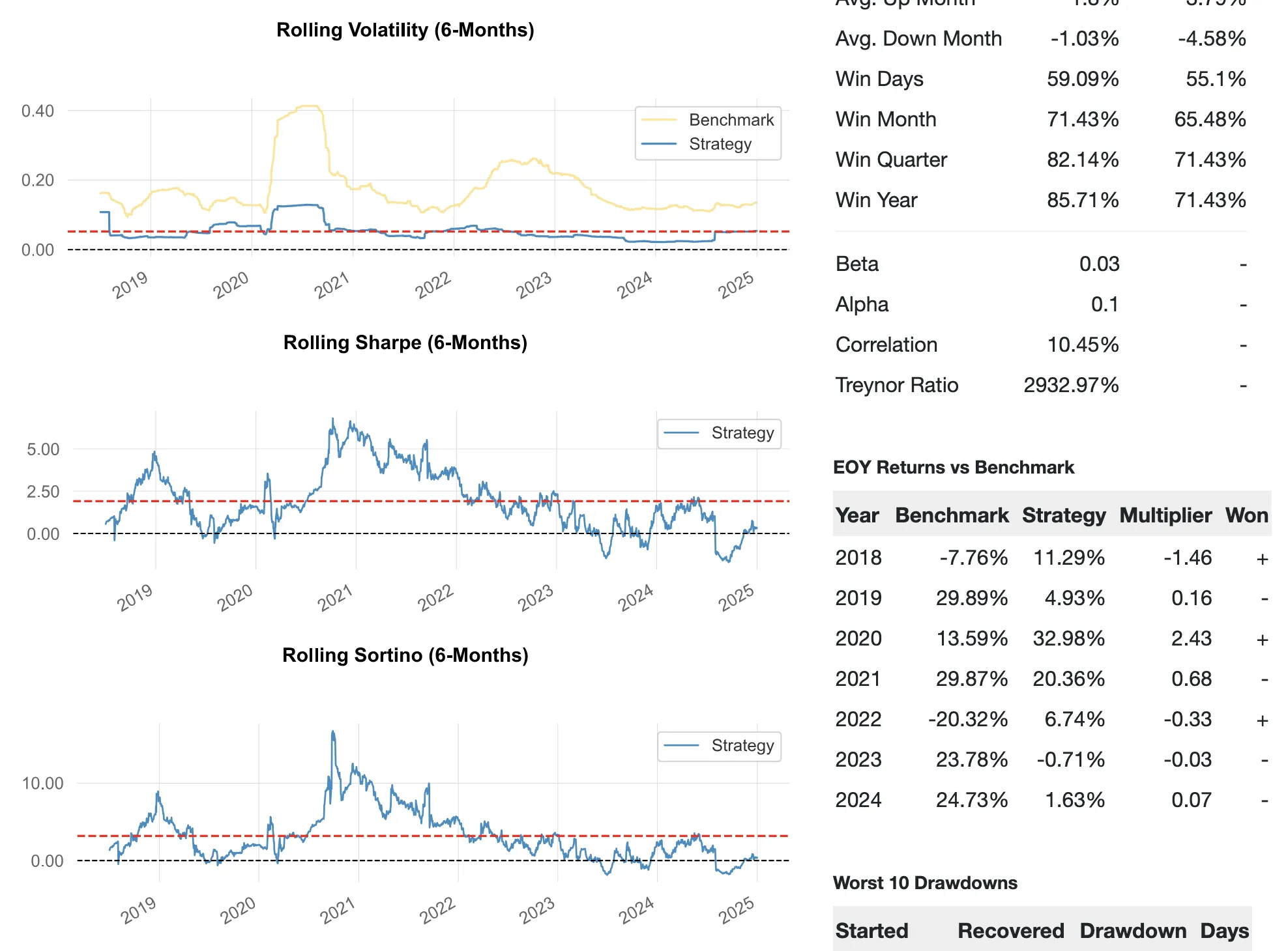
BWB-Cal by Ron Bertino

The BWB-Cal trade was developed by Ron Bertino from Trading Dominion and the trade plan is available in the MasterMind service. This strategy uses longer-dated tenors and does not contain any adjustments. The strategy we traded had additional hedges (2LPs in a third expiration cycle), which were added to mitigate the drawdowns observed during COVID.

Backtest Summary

• Backtest period: 2018-01-01 to 2025-11-11
• Sharpe Ratio: 1.65
• CAGR / Max Drawdown: 10.51% / -6.67%

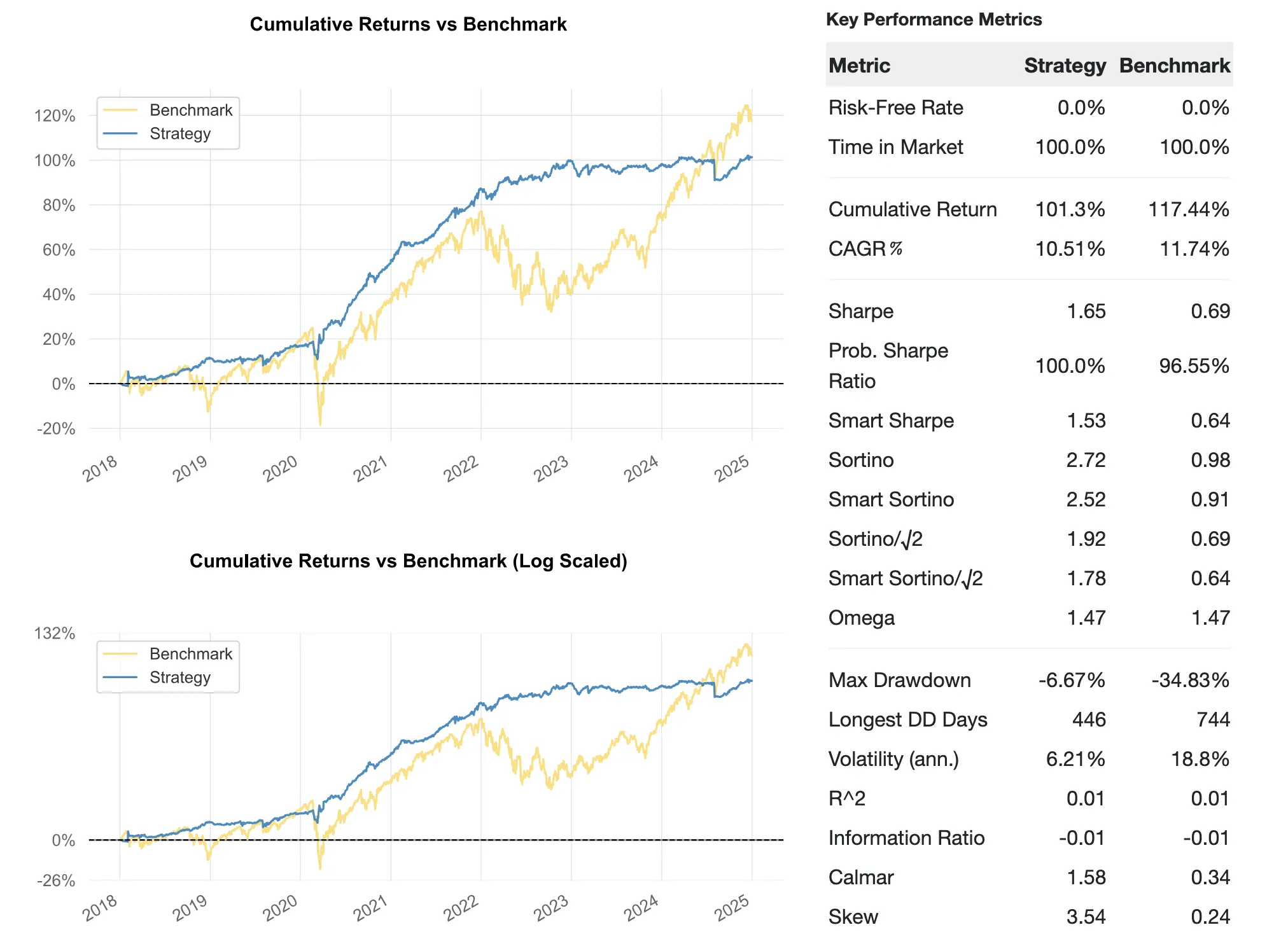
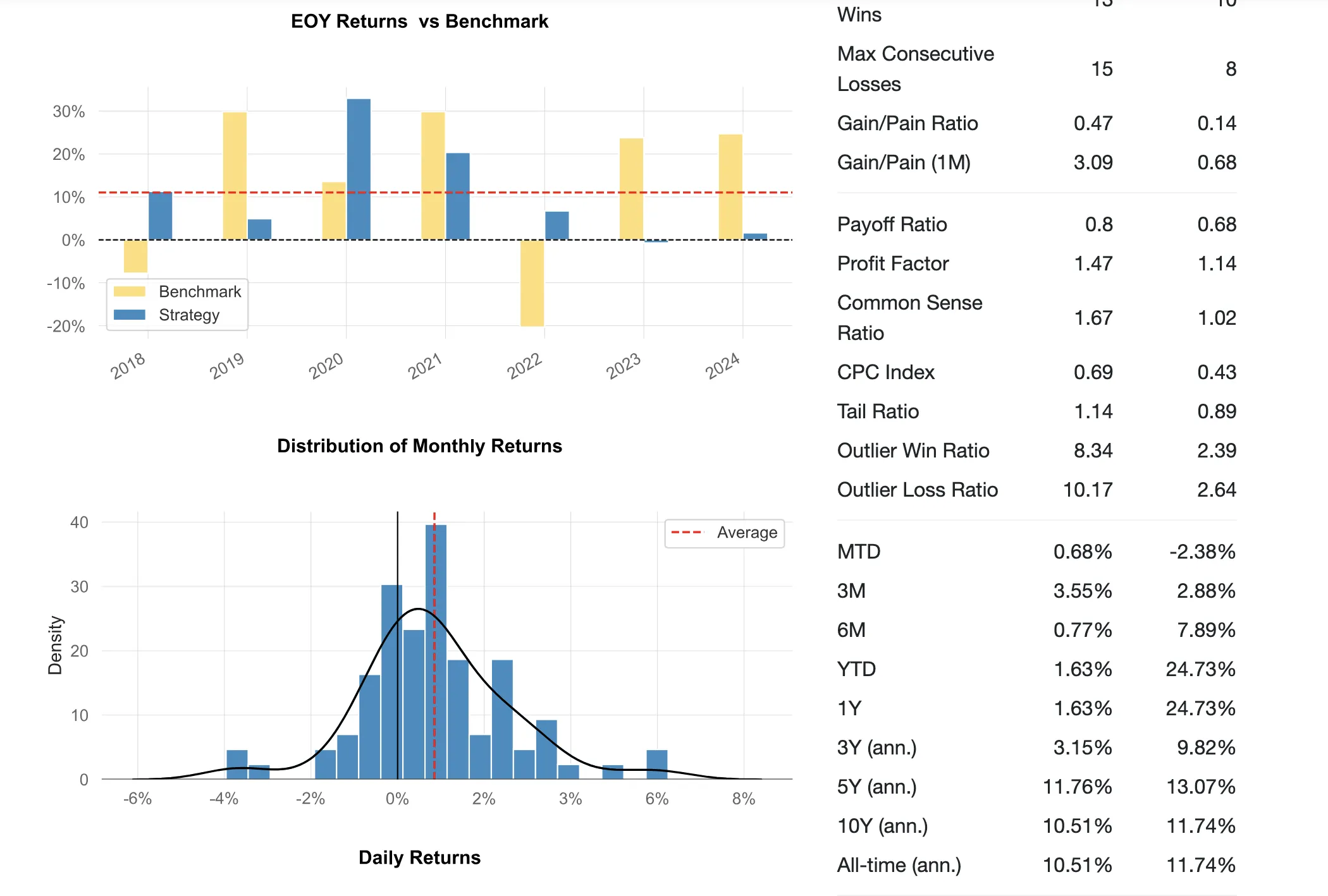
We traded this strategy live between 2022. June and 2023. March. The 2022 performance was convincing but the 2023 performance wiped the previous year's profits. Other MasterMind members at the time achieved similar live-trading performance. To quote Brad: "IV up and Skew up. Double whammy"

The two years of sideways performance confirm that it was the right choice to stop this trade. We attribute the lack of performance to changes in the market dynamics, similarly as we saw it with the NetZero Trade.

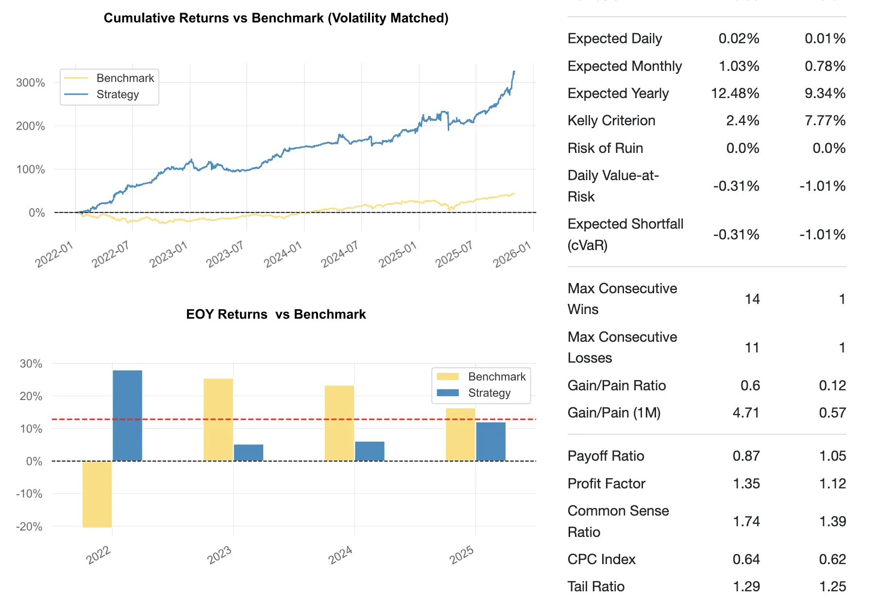
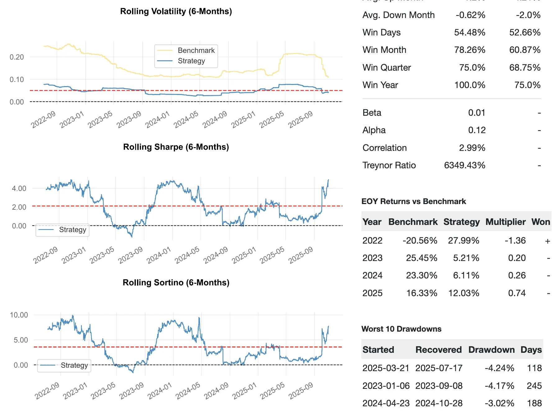
GeneticRhino-25Q4

We believe that optimization and re-optimization is an essential part of every trade lifecycle and, as researchers, our goal is to come up with better performing variant. When it comes to optimization - manual or automated - overfitting is always a risk, but we believe that with proper precautions it can be mitigated. We will use a Genetic Algorithm to find a good-enough solution in a reasonable time-frame. As the name of this section implies: we suggest redoing this optimization at least quarterly.

The original Rhino is a fairly dynamic trade: structures (BWB, PDS, Calendars) are added and removed. This dynamism comes with costs:

• it's more difficult to reason about: one needs to understand multiple structure combinations with varying wing-lengths
• contains more parameters and thresholds to tune.

Therefore, we apply the following simplifications of the trade before optimizing:

• Initiation: The original trade has a fairly complex (VIX-based) leg selection. Our intuition (and later, experience) tells us that the leg selection can be simplified by delta-based rules as delta is derived from volatilities. This can replace the VIX-based wing-width calculation while keeping the same risk profile.
• Adjustments: Layering and adding structures definitely shape the overall delta, but MesoSim supports this natively using the Campaign-style trading. Moving single legs around to adjust delta is a well-known practice, and - we believe - that it can provide a more cost-effective mean to keep the position delta in check.
• Exit: In cases of strongly trending markets it might happen that the underlying leaves the tent completely, rendering the trade's outcome negative. Exiting and re-entering at that stage is a better option than trying to balance deltas using single leg moves.

Taking the above into consideration we're tasked with obtaining the optimal settings for the trade. Our decision space is defined as follows:

Decision Space

Numerical Parameter	Minimum	Maximum	Step
expiration_front_dte	7	100	4
expiration_front_to_back_distance	7	30	1
max_days_in_trade	1	expiration_front_dte	2
lower_long_delta	3	10	1
short_put_delta	lower_long_delta	30	1
upper_long_delta	short_put_delta	50	1
short_cal_delta	15	50	1
delta_adj_threshold_lower (a1)	5	20	5
delta_adj_threshold_upper (a2)	-5	-20	-5
delta_cutoff	max(a1, a2) + 5	max(a1, a2) + 15	1

Categorical Parameter	Values
adjustment_leg_name_lower	short_put / lower_long_put / upper_long_put
adjustment_leg_name_upper	short_call / long_call
lower_cutoff_leg_name	short_put / lower_long_put / upper_long_put
upper_cutoff_leg_name	short_call / long_call

The dumbest (and most thorough) approach is to simply brute-force the expirations, deltas, adjustment thresholds and exit rules. Even with the simplified setup, the total number of combinations are enormous:

648 × 24 × 6440 × 36 × 4 × 4 × 11 × 3 × 2 × 3 × 2 = 22,844,927,508,480 combinations.

We can't tackle this using brute-force, but we can use Genetic Algorithms to find a good-enough solution in a reasonable time-frame.

MesoMiner

MesoMiner is our latest addition to the FundPro offering which is built to tackle exactly this type of problem:

MesoMiner was inspired by Google's AlphaEvolve and blends AI models with evolutionary algorithms to efficiently explore large decision spaces.

As with any optimization (and trade development) process, there is a risk of overfitting. We mitigate this risk by:

• Using an In-Sample (IS) and Out-Of-Sample (OOS) period split (50/50)
• Rely on Deflated Sharpe Ratio to account for the multiple testing bias
• Keeping the original trade structure (BWB + Cal) defined using Min / Max ranges during the leg selection process

You can read more about the IS / OOS split and DSR below.

IS / OOS Split

While doing the IS / OOS split, we take the approach of optimizing in the most recent period (2022-2025) and validating in the older period (2018-2022). Both periods contain market turmoils (e.g. 2020 Covid crash, 2024 VolZilla), sideways and trending markets.

Researchers often set the OOS period is to the most recent period, but our experience is that the benefits of having a recently optimized strategy outweight the drawbacks. Using the older data in the OOS period results in a trade optimized (IS) for the most recent period. It's easy to see that an optimized trade performance will likely be better tomorrow, than 1 or 10 years from now. Since there is no overlap between the two periods, the validation is valid either way.i

Deflated Sharpe Ratio (DSR)

Introduced by Marcos López de Prado and David H. Bailey in The Deflated Sharpe Ratio: Correcting for Selection Bias, Backtest Overfitting and Non-Normality (2014), the Deflated Sharpe Ratio provides a principled way to account for optimization processes.

It adjusts a strategy’s Sharpe ratio for the two forces that typically inflate backtest results: selection bias from testing many configurations, and the non-normal shape of real-world returns.

The key idea is that when a researcher runs a large number of trials, the best-performing Sharpe ratio is almost always upwardly biased. The DSR corrects this by replacing the usual zero-Sharpe benchmark with the expected maximum Sharpe produced purely by chance, a value derived from the distribution of Sharpe ratios across all trials

The Deflated Sharpe Ratio (DSR) is a metric similar to Sharpe, whereas the DSR Probability is the final output of the DSR computation: the probability that the strategy’s Sharpe ratio is truly positive after accounting for multiple trials and the skew and kurtosis of the actual return series.

Optimization results

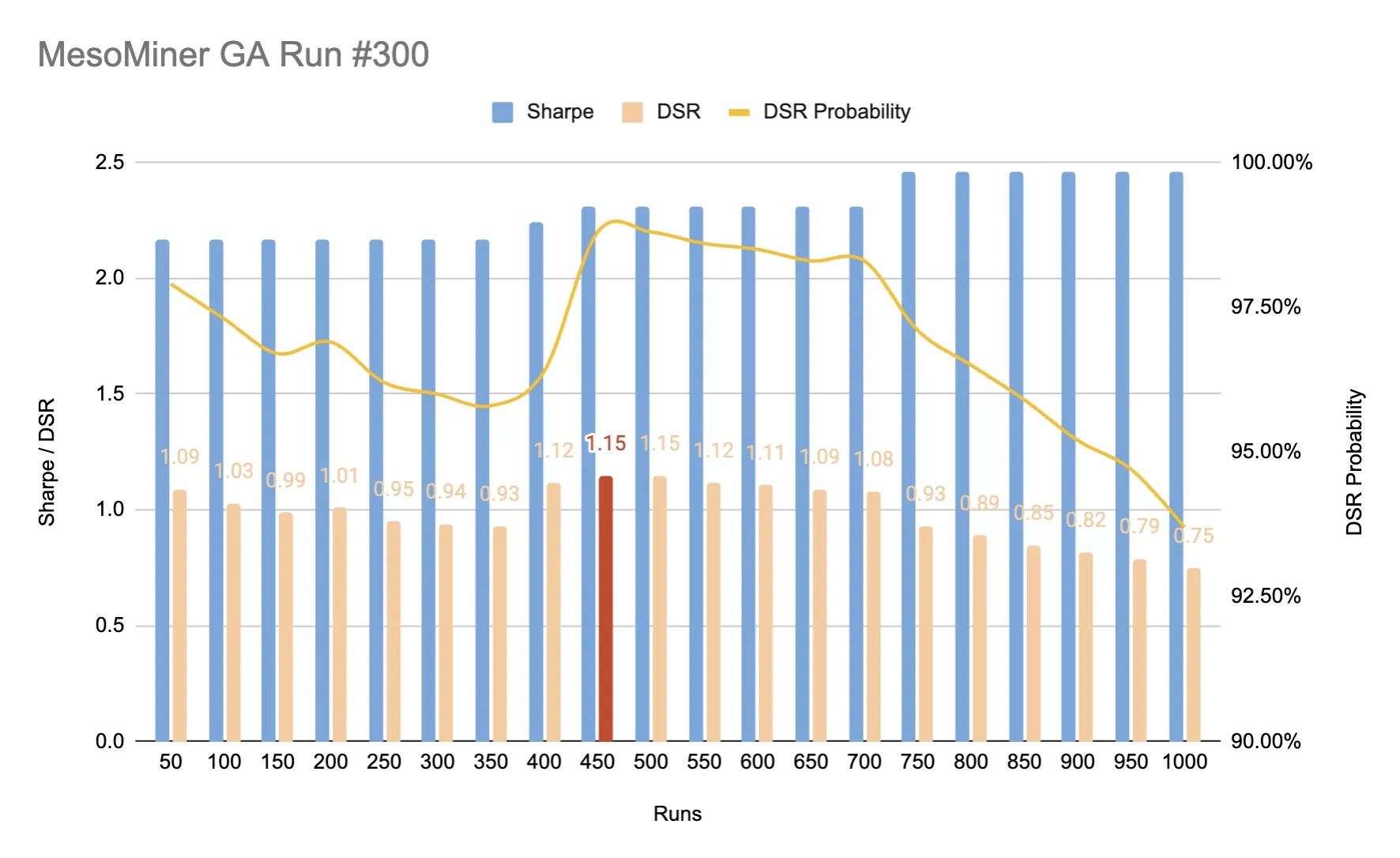
MesoMiner was run with a population size of 50 for 20 generations on the In-Sample period 2022-01-01 to 2025-11-11. The best results (in terms of Sharpe) is reported, whenever a population reaches new highs. We accept the fact that the Sharpe ratio will be optimistically biased / inflated. As the trials grow, the Deflated Sharpe Ratio decreases until a new "best result" is found.

Runs	Best Run In Population	CAGR	MaxDD	Sharpe	DSR	DSR Probability
50	780b6ad8-...	12.2%	-4.2%	2.17	1.09	97.9%
400	da8721df-...	10.1%	-5.2%	2.24	1.12	96.4%
450	7fb14ac4-...	13.1%	-4.2%	2.31	1.15	98.8%
750	bbb95eb2-...	12.5%	-4.4%	2.46	0.93	97.1%

Best In-Sample results by DSR

Besides monitoring the DSR we also track the DSR Probability and aims to pick runs where there is high confidence that the Sharpe is truly positive: cutoff at 95%. Considering the DSR and DSR Probability we pick the best run at the 450 runs mark and we validate this using the withheld, 2018 - 2022 period.

Period	Run	CAGR	MaxDD	Sharpe
IS	7fb14ac4-...	13.1%	-4.2%	2.31
OOS	07763433-...	9.21%	-6.74%	2.2

The Out-of-Sample results confirm that the optimized trade performs well on unseen data, with a Sharpe ratio similar to the In-Sample period. Our expectation is that the trade will perform well in the near future, but re-optimization will be needed as market conditions change.

Optimized Trade Plan

You can study the Strategy Definition in the MesoSim Portal or you can use MesoSim AI Agent.

Here is a brief summary of the optimized trade plan:

Underlying: SPX.

Expirations:

• exp1 (front): target ≈ 99 DTE for the entire BWB and the short call.
• exp2 (back): target ≈ 110 DTE (Min=110), used for the long call hedge.

Structure:

• BWB:
  • short_put (exp1): Qty −2, Δ≈22.
  • lower_long_put (exp1): Qty +1, Δ≈6. Max(Δ) dynamically capped by per-contract delta of the short put.
  • upper_long_put (exp1): Qty +1, Δ≈46, with a dynamic Min(Δ) tied to the short put’s per-contract delta; Max=50.
• Call diagonal:
  • short_call (exp1): Qty −1, Δ≈24, Max(Δ)=50.
  • long_call (exp2): Qty +1, Δ set to abs(pos_delta) at selection time to neutralize with a back-month long leg

Entry: Daily, 30 min after open. Up to 12 simultaneous positions, with 6-day entry staggering → campaign deployment to smooth path risk. No gating conditions.

Adjustments: Daily, 60 min after close. Delta guardrails with surgical rolls:

• If pos_delta > 5: move upper_long_put (front-month wing) to a new strike as such that the position delta becomes 0.
• If pos_delta < −5: move short_call similarly, re-setting position delta to 0 by shifting the short call’s strike.

Exit: Daily, 30 min before close. Max Days in Trade: 53. Hard exit conditions (any hit → close):

• Downside breach: spot < short-put strike
• Upside breach: spot > back-month long-call strike
• Greeks: abs(pos_delta) > 16
• No explicit PT/SL; exits are path-driven by barriers + delta.

Further work

• Calendarized structures can "sink" when volatility becomes unfavorable for the position. With MesoSim-v3.0 such cases can now be detected and acted upon by using the Options Valuation Model.
• Margin to Equity (MtE) and Equity to Vega ratios can be incorporated to the original Rhino plan to better match Bruno's style of trading. The required tools are already provided by MesoSim.
• Slippage modeling can be enabled to better capture the real-life trading costs. Our experience is that the genetic variant can be filled using two orders, each slipping by 5 cents from mid-price (SPX).

Do you have other ideas or suggestions?
Please leave a comment below!

---

Conclusion

Rhino is a family of related broken‑wing butterfly income trades that have evolved over nearly a decade. The latest rules of the original trade (from 2023) still hold up in today's market, providing reasonable performance.

We hope our GeneticRhino-SPX-25Q4 implementation will hold up and provide good performance for the next few months. We are sure, however, that re-optimization is an integral part of trade development process and the trade can benefit from it as market conditions are changing.

Both trade plans are readily available for live and paper trading in MesoLive and can be further customized in MesoSim.

Some of the historical variants shown later in this article have not performed well in the recent markets. That’s not a criticism of their original designers; it just illustrates what Bruno Voisin keeps repeating:

Adapt or die.

Acknowledgements

We would like to thank Bruno Voisin for his pioneering work on the Rhino trade and for making much of his material publicly available. His support throughout the development of this article has been invaluable.

We also thank Claudio Valerio and Rafael Munhoz for their feedback on the drafts of this article.