Portfolio Construction Methods

Overview
Over the last two years, we have shared numerous backtests featuring public options trading strategies (such as NetZero, Boxcar, or Weekend Effect), strategy variants contributed by our customers (Volatility Hedged Theta Engine, Relaxed SuperBull trade), and built-in strategy templates that turned out to be good starting points (trailing stop, 0DTE-IC).
These income strategies cover a wide range of moneyness and time to maturity. Some stand out, others are just average and some are not performing well currently.
It is well known that diversification helps build better investments.In this article, we will explore how Equal Weighting and Modern Portfolio Theory might help improve investment performance.
Setup
Time Period
In our experiment we will cover the last 4 years of historical data: 2020. 06. 31 - 2024. 06. 31. The S&P 500's performance from mid-2020 to mid-2024 can be characterized by a strong initial recovery, a period of volatility, and
subsequent stabilization and growth.
The time period is purposely selected to exclude the COVID crash because the majority of the strategies exclude the hedging component. Hedging should be researched separately to find a strategy that meets the investor’s risk tolerance.
Strategies
All strategies are compounding and traded using SPX Options.
| Backtest | Run | CAGR | Max DD | Sharpe |
|---|---|---|---|---|
| quantpedia-seasonality-vrp | Run | 31.39% | -16.77% | 1.85 |
| 45dte-short-put-trailingstop | Run | 81.99% | -32.14% | 1.65 |
| weekend | Run | 14.65% | -12.56% | 1.62 |
| thetaengine-volhedged | Run | 48.58% | -27.13% | 1.44 |
| boxcar-ng | Run | 60.14% | -65.9% | 1.1 |
| strangle-adjusting | Run | 20.44% | -32.74% | 0.89 |
| superbull-relaxed | Run | 32.33% | -59.2% | 0.84 |
| 0dte-ic | Run | 14.09% | -25.7% | 0.75 |
| netzero | Run | 14.51% | -39.89% | 0.6 |
| 120dte-ic | Run | 19.34% | -75.23% | 0.59 |
Q-API: The Quantitative API
To analyze the portfolio construction we will use Q-API, our free quantitative API providing:
- Tearsheet Generation
- Portfolio Analytics from Strategy Returns
- Trading calendars
Read the details in the related blog post.
Today we are extending Q-API’s functionality with Portfolio Optimization capabilities combining PyPortfolioOpt’s Mean Variance Optimizer with our proprietary walk-forward optimizer.
To make the research reproducible we are publishing our calculations on Github. You can also open it in Google Colab directly.
Our retail customers can reproduce the results of the notebook by manually downloading the NAV export for each run and uploading it to Google Colab’s drive.
While the public Q-API is free to use for our customers (within our reasonable use policy), MesoSim APIs are only available via our FundPro Plan. The NAV files in the example notebook are loaded through the MesoSim API.
If you are a retail customer looking to recreate the steps here, please consult the following notebook on how to load the NAV files in the correct format.
If you would like to use Q-API at scale or MesoSim API please reach out to us at [email protected].
Correlations
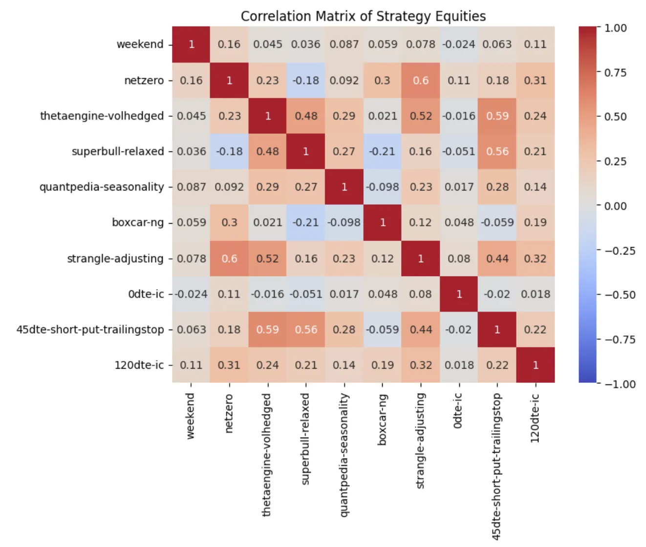
To validate that the strategies are independent of each other, the correlation of log returns can be used. Ideally, the strategies included in a portfolio should have low correlation (<0.3).
We validate this by loading the NAV exports into a DataFrame (merged_df), calculating the respective log returns, and showing the correlation matrix with the help of Pandas and Seaborn:
log_rets = np.log(merged_df).diff().dropna()
correlation_matrix = log_rets.corr()
plt.figure(figsize=(8, 6))
sns.heatmap(correlation_matrix, annot=True, cmap='coolwarm', vmin=-1, vmax=1)
plt.title('Correlation Matrix of Strategy Equities')
plt.show()
Portfolio Construction
Equal Weighting
Equal portfolio weighting is a simple and straightforward investment strategy where an investor allocates an equal amount of capital to each asset within a portfolio. This means that each asset has the same weight or proportion of the total portfolio value, regardless of the asset's market capitalization, risk, or expected return.
Using the previously built DataFrame, we combine the NAVs and show the tearsheet.
total_capital = 100000
num_assets = len(merged_df.columns)
equal_allocation = total_capital / num_assets
portfolio = equal_allocation * merged_df

summed = pd.DataFrame(portfolio)
summed["sum"] = summed.sum(axis=1)

display_tearsheet(Q_API_INSTANCE, API_KEY, summed, 'sum')
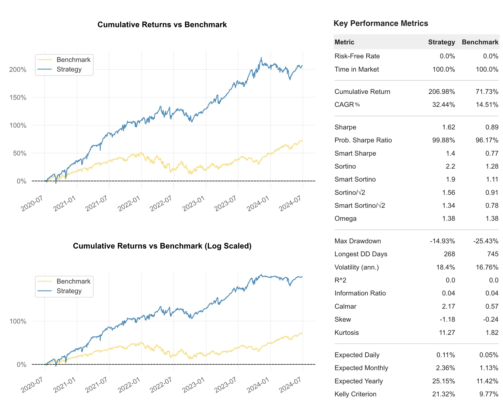
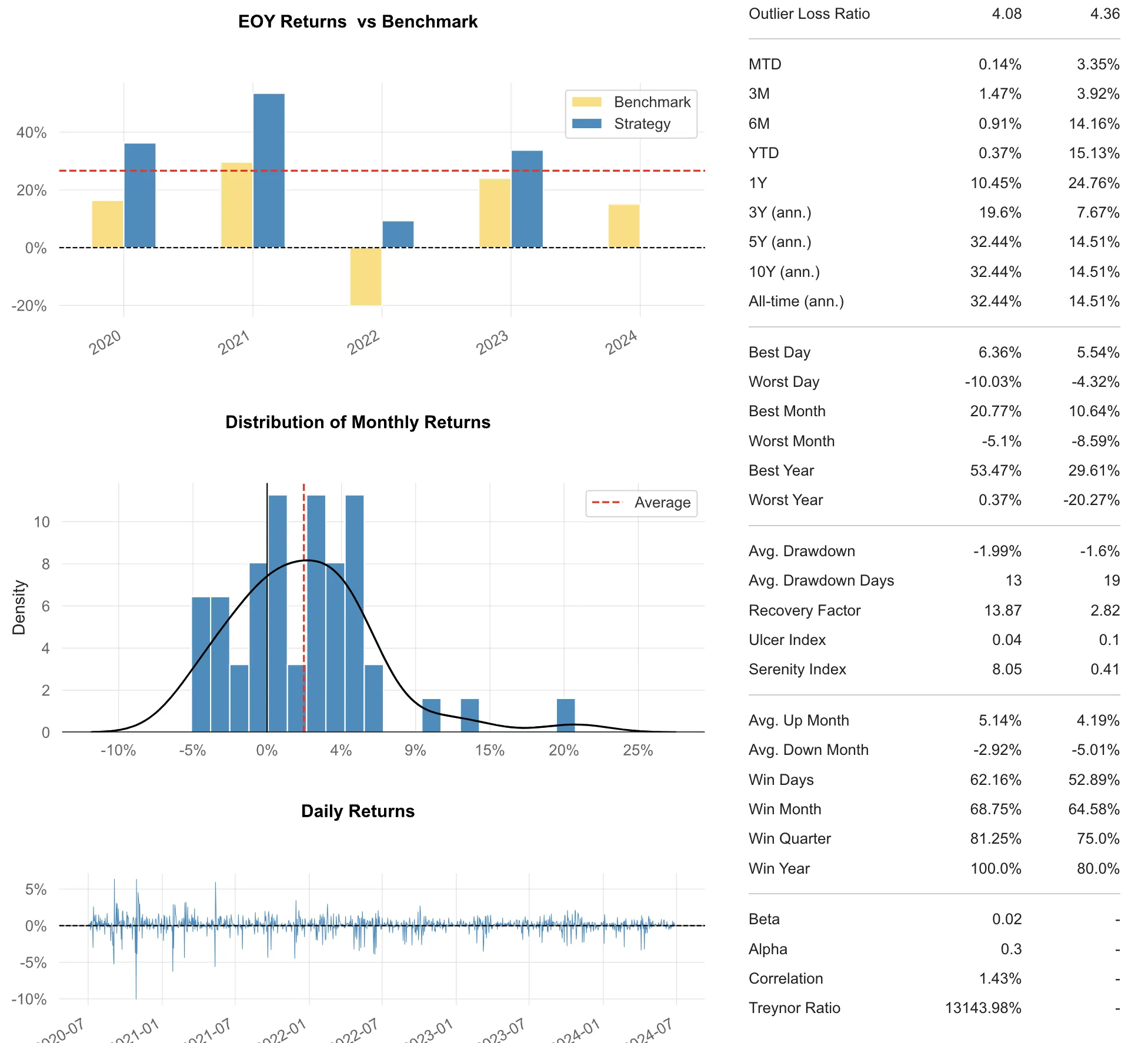
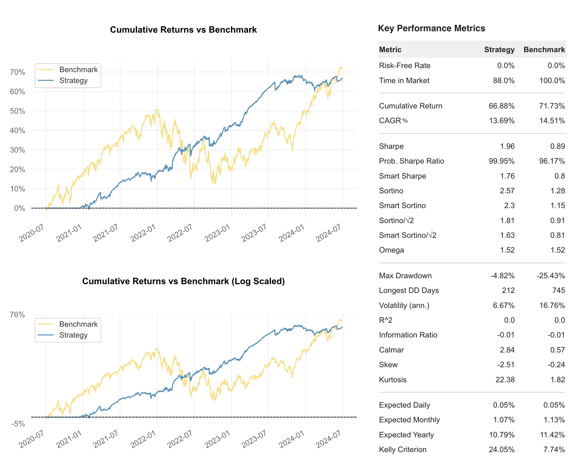
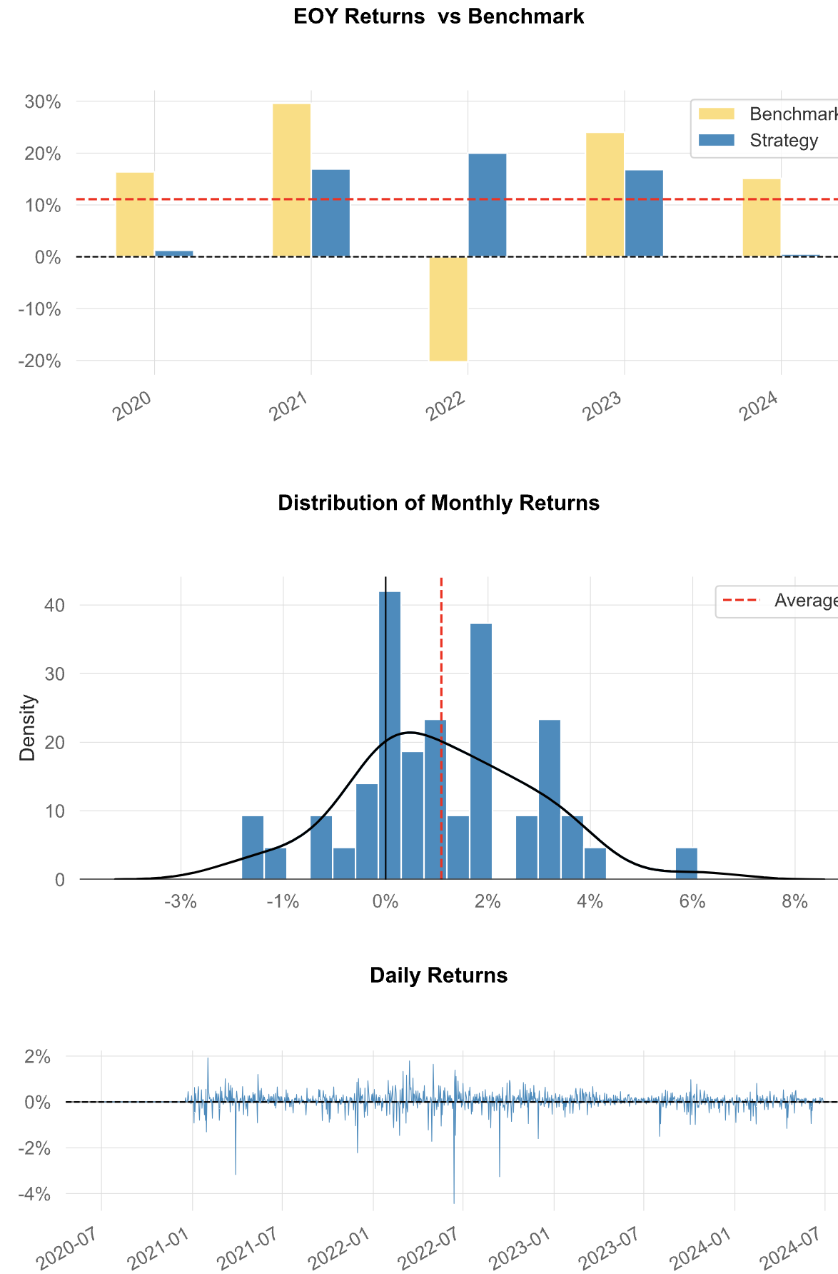
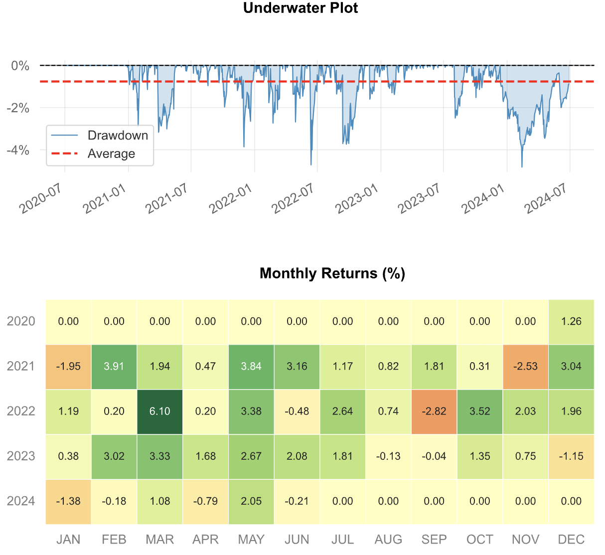
Observations
While the combined portfolio’s Sharpe ratio is a respectable 1.62, it ranks third when compared to the individual strategy performances:
- Sharpe 1.85: Quantpedia-seasonality-vrp
- Sharpe 1.65: 45dte-short-put-trailingstop
- Sharpe 1.62: Weekend and Equal Weight Allocation
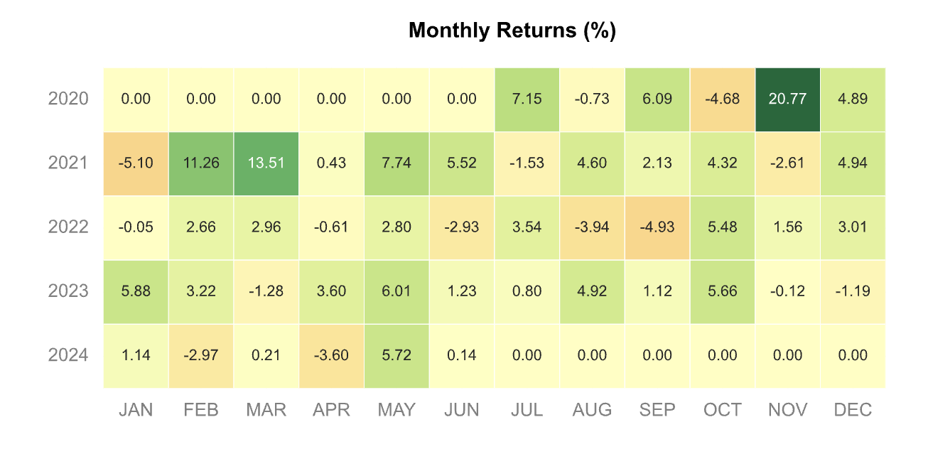
We note that 2024 is not a very successful year for the combined strategies, mostly due to the underperformance of NetZero and 120DTE IC strategies.
Grid Search with Equal Weight Allocation
With 10 different strategies, it is possible to compute all the combinations of the strategies while sticking to the equal allocation strategy. The unique combinations for 10 strategies are 1,023 if we allow strategies to be combined without any restrictions regarding the traded strategy count.
Having all the combinations allows us to get a sense of the highest Sharpe ratio possible with the equal allocation setup. However this approach is impractical for trading as it optimizes on all the data. We can’t apply the obtained ideal weight to the past returns, as it would cause look-ahead bias.
It should be noted that if we allow fractional allocation (just as is done in mean-variance optimization), the search space explodes, and grid search would no longer be feasible.
Results
After completing the 1,023 runs, we visualize the Sharpe ratio as a function of the number of strategies in the portfolio. You can find the further run details in the notebook.
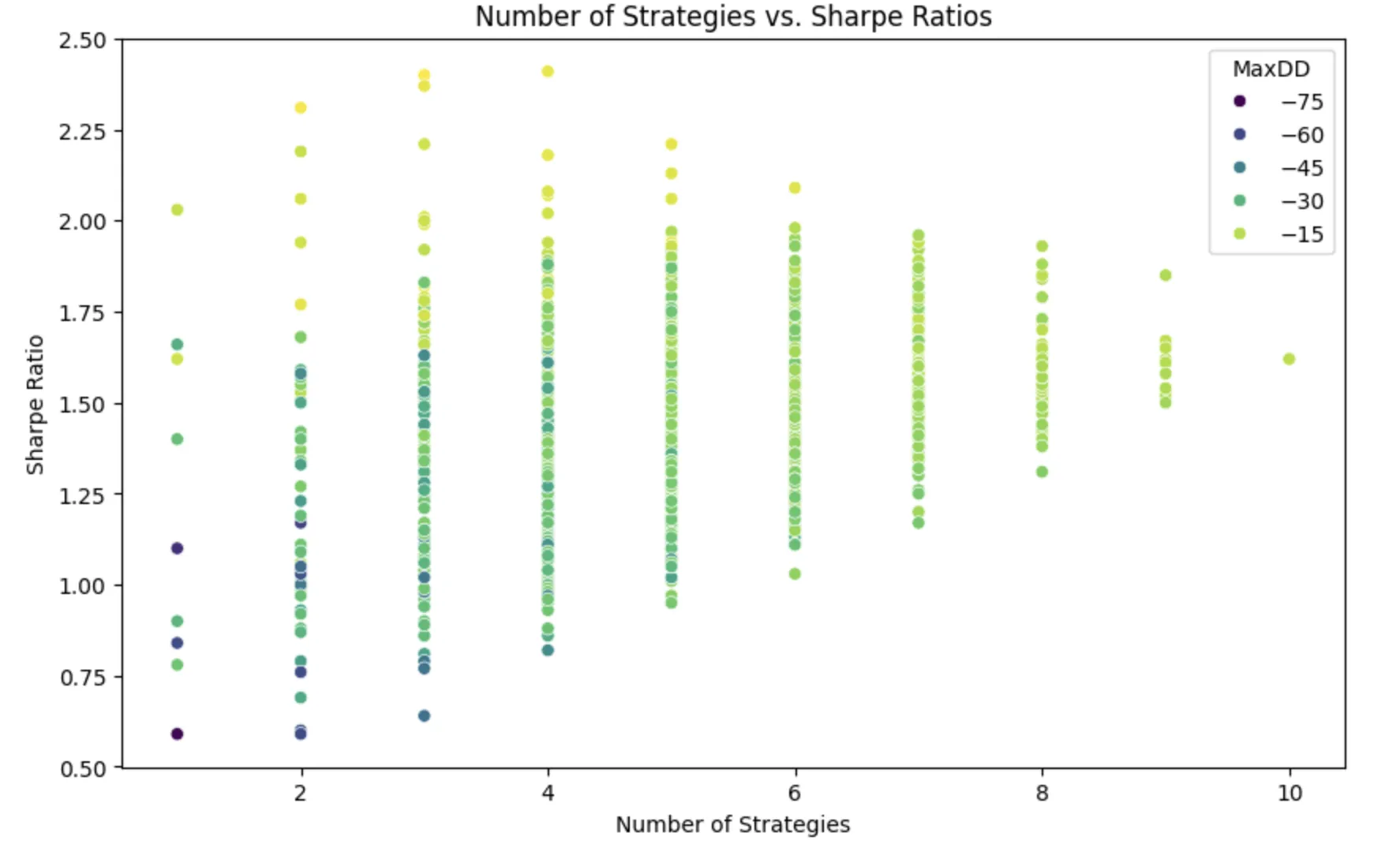
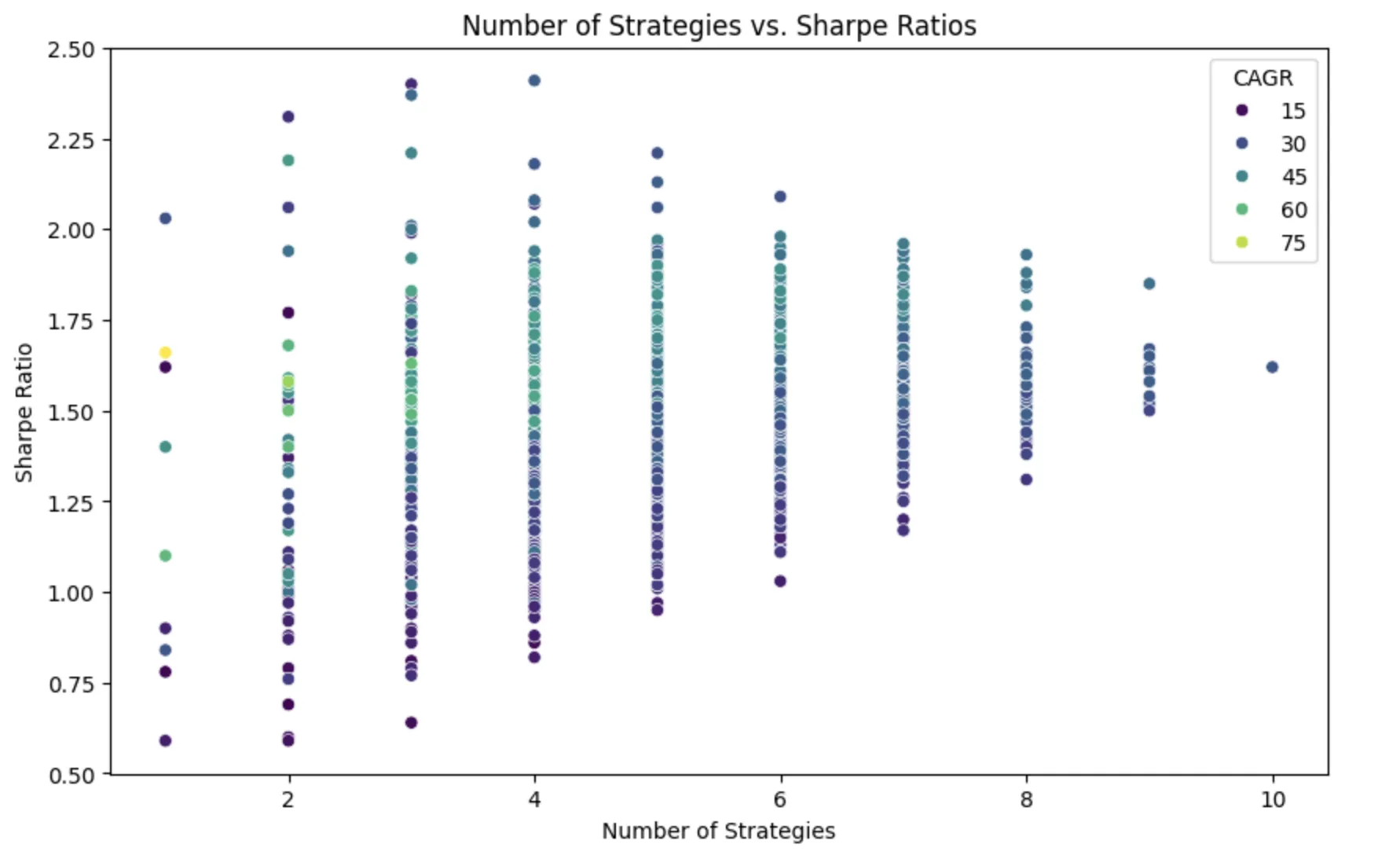
The highest ranking runs are:
- Sharpe 2.41:
weekend + quantpedia-seasonality + 0dte-ic + 45dte-short-put-trailingstop - Sharpe 2.40:
weekend + quantpedia-seasonality + 0dte-ic - Sharpe 2.37:
weekend + quantpedia-seasonality + 45dte-short-put-trailingstop
The equal-weighted portfolio across all the strategies is represented by the right-most dot in the charts, with 10 strategies allocated.
Observations:
From this experiment, we conclude that the equal-weighted portfolio using all the instruments is in the middle of the achievable performance.
Modern Portfolio Theory
To improve on the previous results, we will apply Modern Portfolio Theory’s Mean-Variance Optimization with walk-forward optimization. In the Q-API, we combine PyPortfolioOpt’s mean-variance optimizer with our proprietary walk-forward optimizer. The end result is a constantly optimized set of weights that can be used to rebalance the portfolio. The user can specify the length of the windows (folds) used in walk-forward. The rebalancing interval is set to daily.
Mean-Variance Optimization (MVO) is a mathematical framework used to construct investment portfolios that aim to maximize expected return for a given level of risk, or equivalently, minimize risk for a given level of expected return. This concept was introduced by Harry Markowitz in his groundbreaking work on Modern Portfolio Theory (MPT) in the 1950s.
Walk-forward optimization is a robust technique used in financial trading strategies to evaluate and improve the performance of trading models. It involves repeatedly optimizing and testing a trading strategy over different segments of historical data, aiming to better simulate real-world trading.
Optimization targets
Optimization mode
The mean-variance optimizer currently supports Sharpe Maximization and Volatility Minimization objectives. During Sharpe maximization, the optimizer expects future returns, something hard to come by. To simply bridge the gap, we provide past returns as proxies for future returns. However, expectations must be set correctly: past returns rarely predict future returns. Therefore, we may be better off with the minimizing volatility target. Volatility targeting is a well-researched topic and can be practically applied to portfolio construction.
Walk-forward window
The second parameter of the optimizer is the window size for the walk-forward folds, specified in trading days. The longer the period, the more stable the results will become, but the response/lag to changes will generally be longer. We will scale this parameter from 20 (1 trading month) to 240 (approximately 1 trading year).
Number of assets in protfolio
In practice, optimizers return weights for all instruments. Our approach is to pick the 5 highest-ranking weights and make allocations accordingly. We arbitrarily choose 5 with the aim of not having too many positions allocated below 10%. We can also tell the optimizer to show the full allocation by setting the top allocation (topAlloc) equal to the number of items in the portfolio. In all cases, we need to ensure that we have enough capital to trade the scaled portfolio.
Walk-Forward Results
The following table shows the Sharpe ratios for each window and optimization target. Please find the respective code generating this result in the notebook.
| Walk-forward window | MVO/Max Sharpe | MVO/Min Volatility |
|---|---|---|
| 20 | 1.3 | 1.87 |
| 40 | 0.76 | 1.48 |
| 60 | 0.72 | 1.78 |
| 120 | 0.98 | 1.96 |
| 240 | 1.14 | 1.88 |
Observations
The preceding table summarizes the achieved Sharpe ratio as a function of optimization type and walk-forward window.
It is apparent that the volatility minimization target outperforms the Sharpe maximization targets by a large margin (using Sharpe as a metric).
We also conclude that nearly all min-volatility walk-forward results achieve higher Sharpe ratios than the equal allocation portfolio or the individual strategies.
The highest ranking
The highest-ranking portfolio from the above experiment was the min-volatility targeted optimization with a 120-day window when the Sharpe ratio is used as a benchmark.
To study the allocation over time, we can use the walkforward-weights endpoint to get the weights.
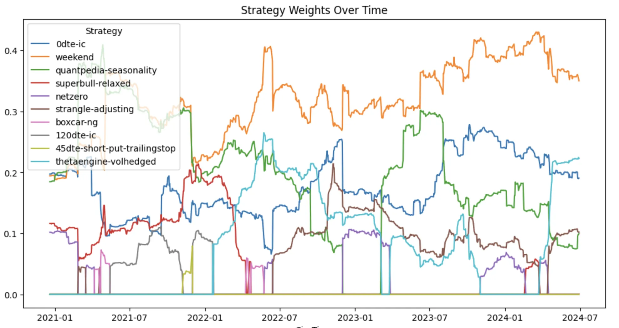
Observations
- The Weekend trade has the largest allocation, around 40%.
- The Weekend trade occupies the highest allocation for almost the entire period.
- The top performer strategy (quantpedia-vrp) has around 10% allocation.
- Recently, the ThetaEngine-Volhedged received a 20% allocation.
- The two underperformers for 2024 (NetZero and 120DTE-IC) are mostly excluded in that year.
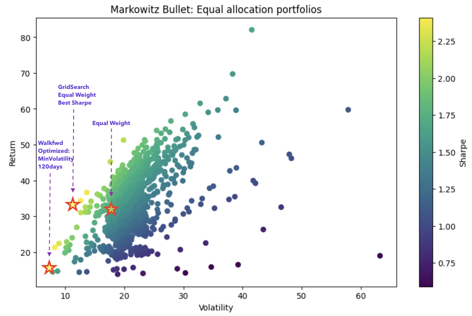
Overview
In order to visualize the above experiments we’ll be using Return / Volatility graphs used in visualization of Efficient Frontier. The Grid Search runs nicely showing the Markowitz Bullet Shape.
It is apparent that the walk-forward optimization with target of Minimum volatility achieved it�’s optimization target.
Conclusion
Modern Portfolio Theory’s Mean Variance Optimization with Volatility Minimization target managed to build a portfolio that has a very low variance and outperforms the Equal Weight allocation.The Q-API can be now effectively used to find weights for any portfolios.
For the fine details please refer to the Colab (ipython) Notebook.
| Notebook | Link |
|---|---|
| Portfolio Optimization notebook | |
| Manually downloaded NAV processor notebook |
Acknowledgements
We would like to thank Robert Martin for creating PyPortfolioOpt.Awesome project with great quality code!