The Weekend Effect in options refers to the tendency of options prices to decrease more over the weekend than in their respective weekday period.
Traders aware of the weekend effect can potentially profit by selling short-term options on Friday and buying them back on Monday at a lower price.
However, this strategy also comes with risks, such as unexpected market events that could cause a significant change in option prices over the weekend. Therefore, it is strongly suggested (mandatory) to pair this trade with a hedge. We will cover hedging strategies in a later article.
The validity of this hypothesis can be evaluated using MesoSim through a series of straightforward tests, which we are undertaking in the subsequent section of this article.
The original trading rule is defined in Euan Sinclair’s book:
"On a Friday, sell the options that expire the next Monday."
Based on this guidance, our backtest trading rules are as follows:
Find next Monday's or Tuesday's expiration
Enter trades using the chosen expiration on Friday, 15 minutes before close
Exit trades on Monday or Tuesday, 15 minutes after the open
note
The Tuesday expiration selection and Exit rules are present so that we can cover long weekends. In case of normal weekends, the Monday expiration and exit should be used.
For demonstrational purposes, we will be using short puts and strangles to showcase this trade. It should be noted though, that the strategy should work with more complex structures, such as butterflies and iron condors.
We set the strategy to enter a position on a Friday and exit on Monday by using the following conditions in the Strategy Definition.
In the Expirations section, we specify that expirations will be selected between three and four DTEs, targeting 3. This enables trades entered on Friday and kept until Monday or Tuesday (in case of a long weekend).
The Entry schedule is set to enter the trade each Friday 15 minutes before market close, and the Exit set to exit the trade the next trading day, 15 minutes after the market opens.
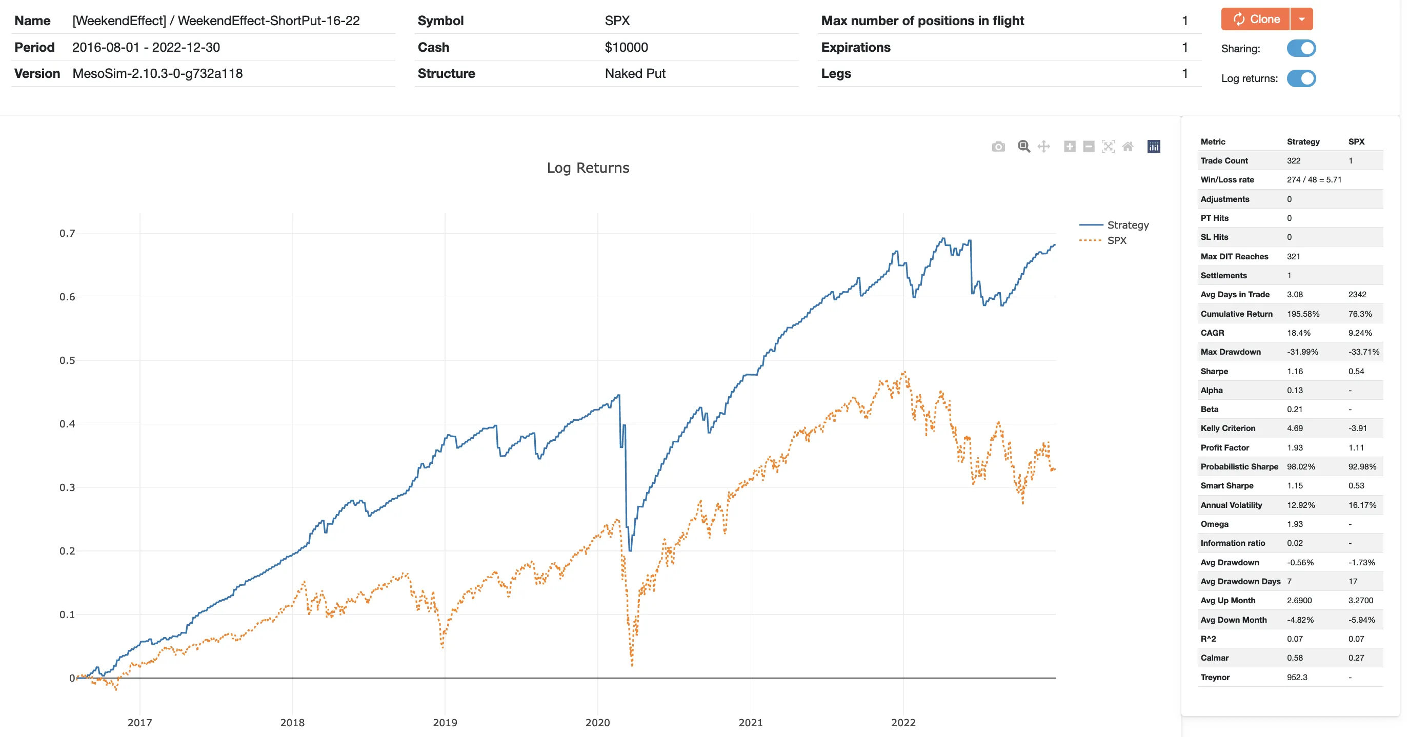
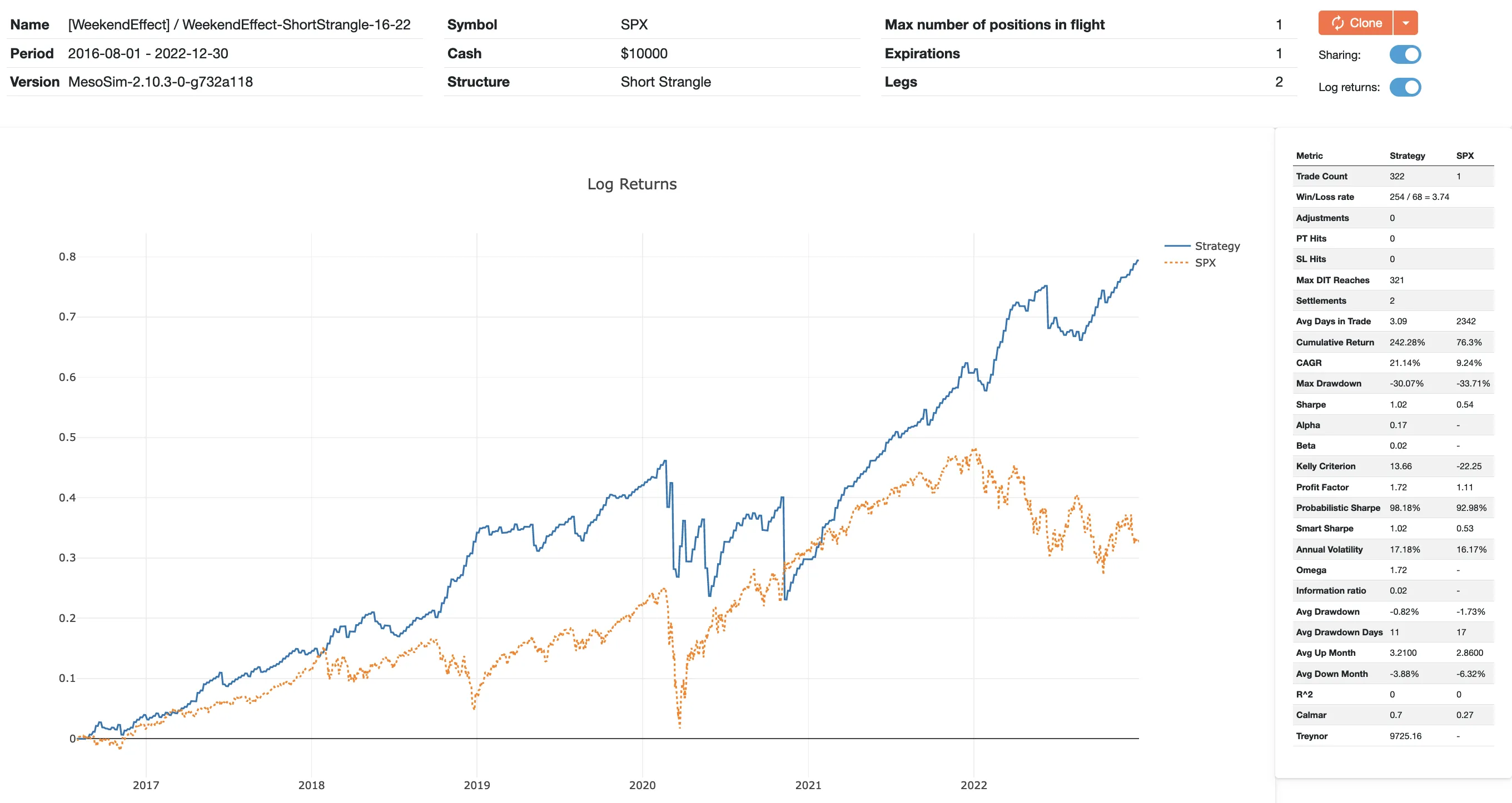
While we reduced the time spent in the market the returns are outperforming a simple S&P buy-and-hold strategy with a great margin: CAGR is doubled while the Max Drawdown stayed the same.
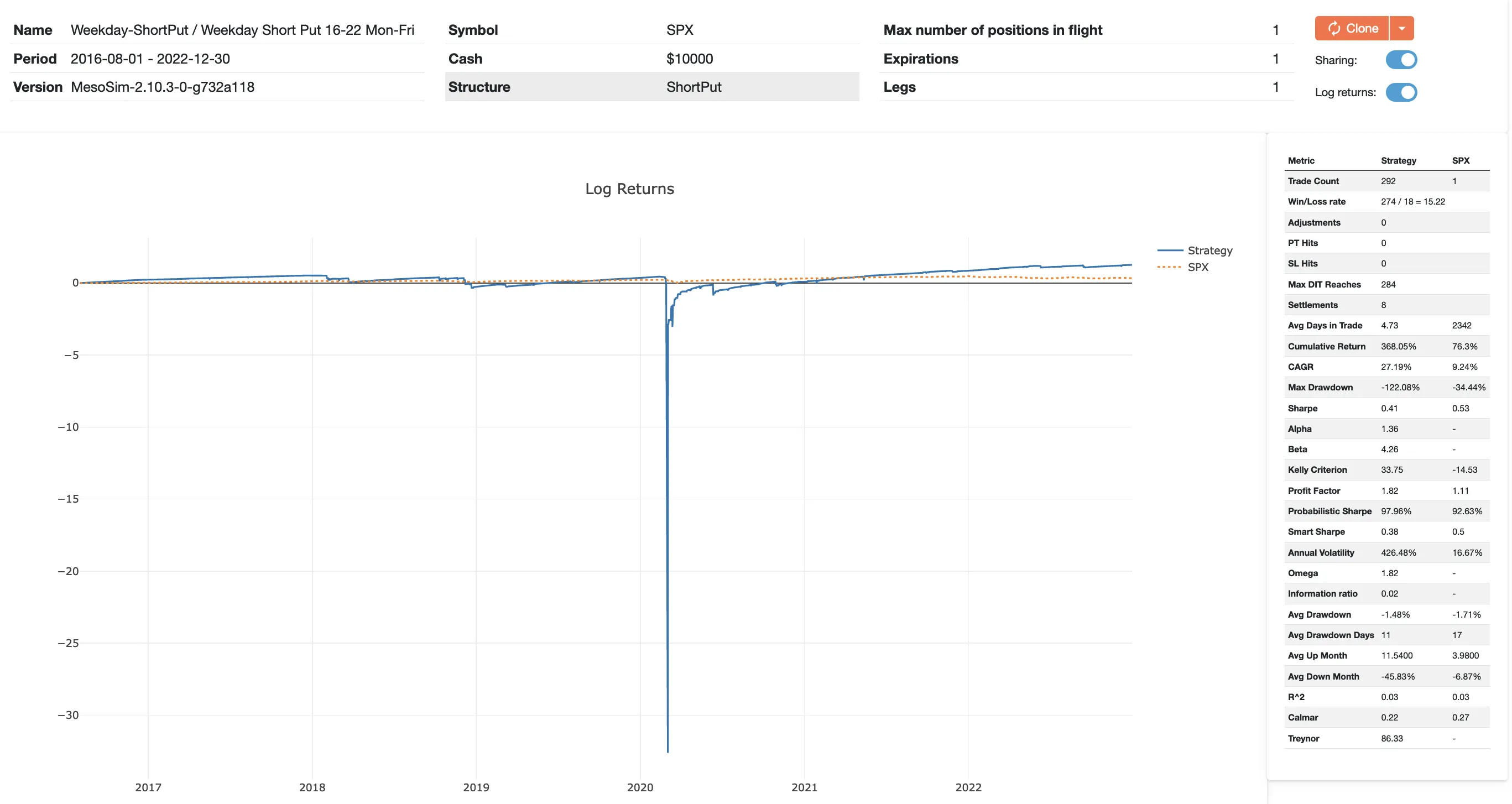
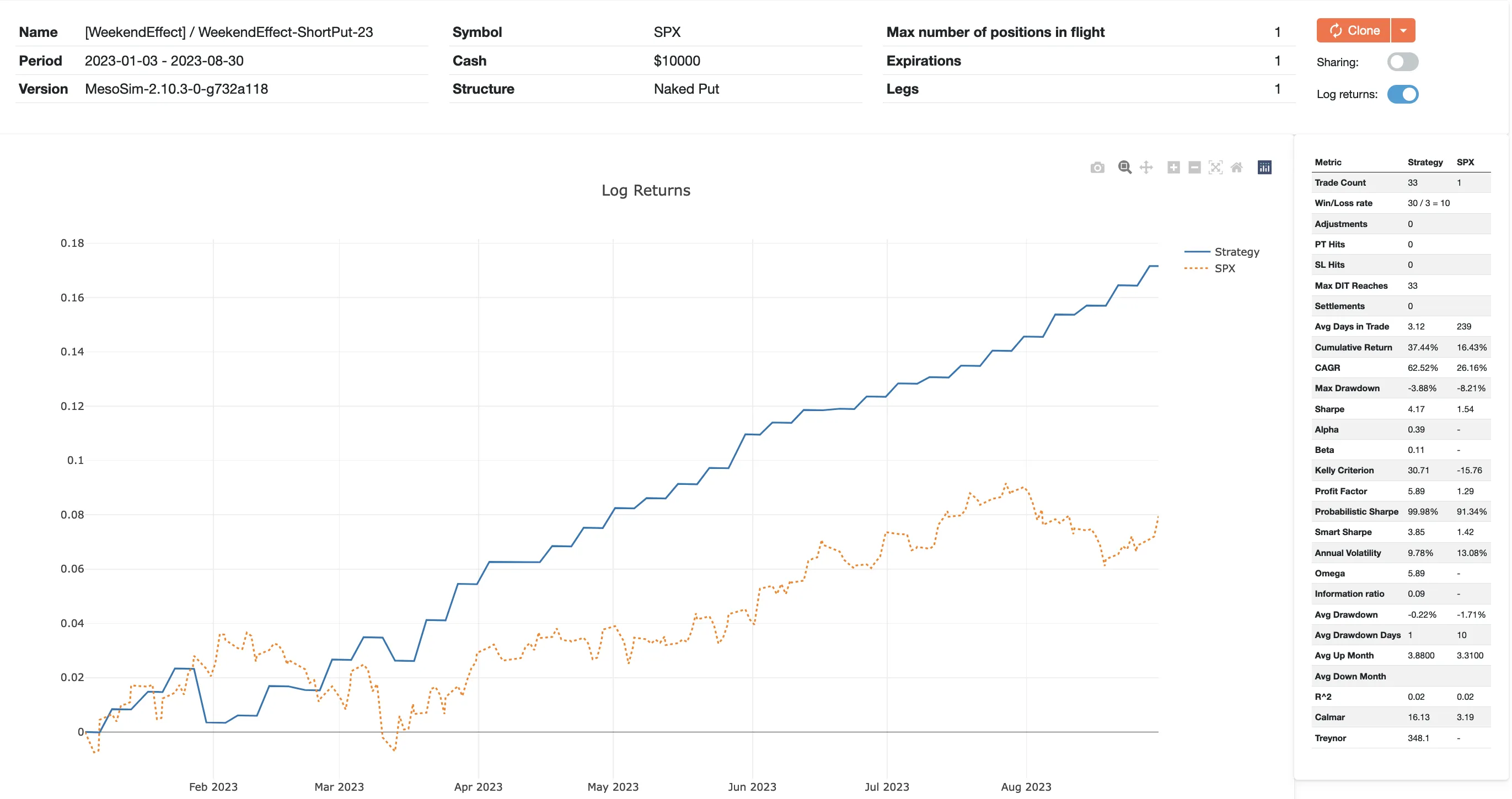
To validate the existence of weekend premium, we modify the backtest’s entry and exit schedule to run to cover the opposite timeframe: Mondays to Fridays (4 DTE short put).
The strategy multiple times has drawdowns above 50%, including (but not limited to) the Covid crash period.
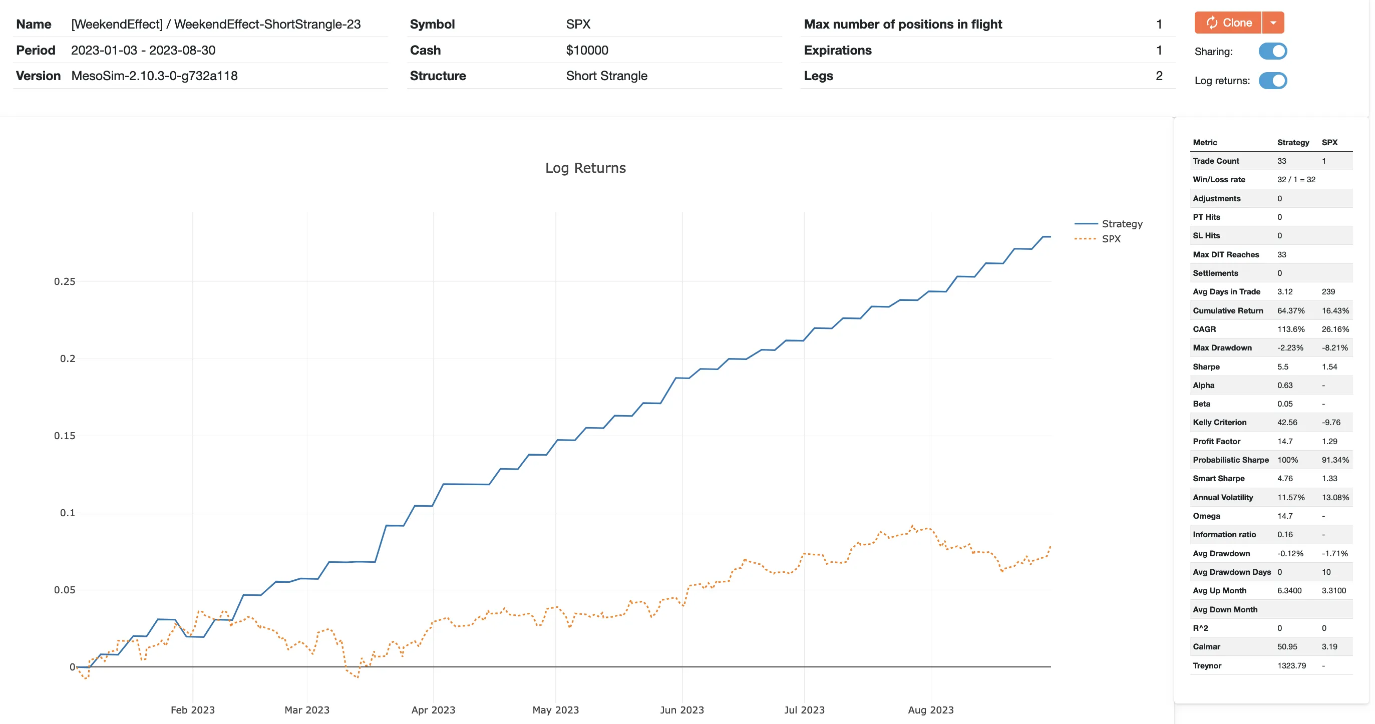
While the Short Put setup meets the Weekend Effect's instructions (sell options on Friday) and shows the effect in its purest form, it is possible to improve the strategy by selling more options:
If we sell Calls as well as Puts we end up having a Short Strangle structure. The collected premium is increased, therefore we expect
larger returns. Since there is more risk on the downside, selling Calls likely won't increase our risk exposure.
Our analysis confirms the significance of the Weekend Effect when the strategy is backtested on S&P Index Options (SPX). Not surprisingly, the Strategy suffers its largest drawdowns during crash situations, such as COVID. Therefore, this (and any other option selling strategy) should be traded when adequate hedging is in place.
We would like to thank Euan Sinclair for spreading his knowledge via his excellent books and courses!
The Short Strangle version of the Weekend Effect is available in MesoSim as a built-in template, named: [WeekendEffect]
MesoSim v3 Migration Note
This article was originally written for MesoSim v2. The examples and terminology have been updated to match the MesoSim v3 Strategy Definition format. For details, see the MesoSim v3.0 release announcement and the v2→v3 migration guide. The performance metrics, described behavior, and referenced run results reflect the original v2 behavior. If you rerun the referenced strategies on MesoSim v3, results may differ slightly due to behavioral changes in the simulator.
Selling put options is akin to operating an insurance business:
the option seller is rewarded with the premium (option price) in exchange for taking the risk of assignment if the market moves below the strike price at expiration.
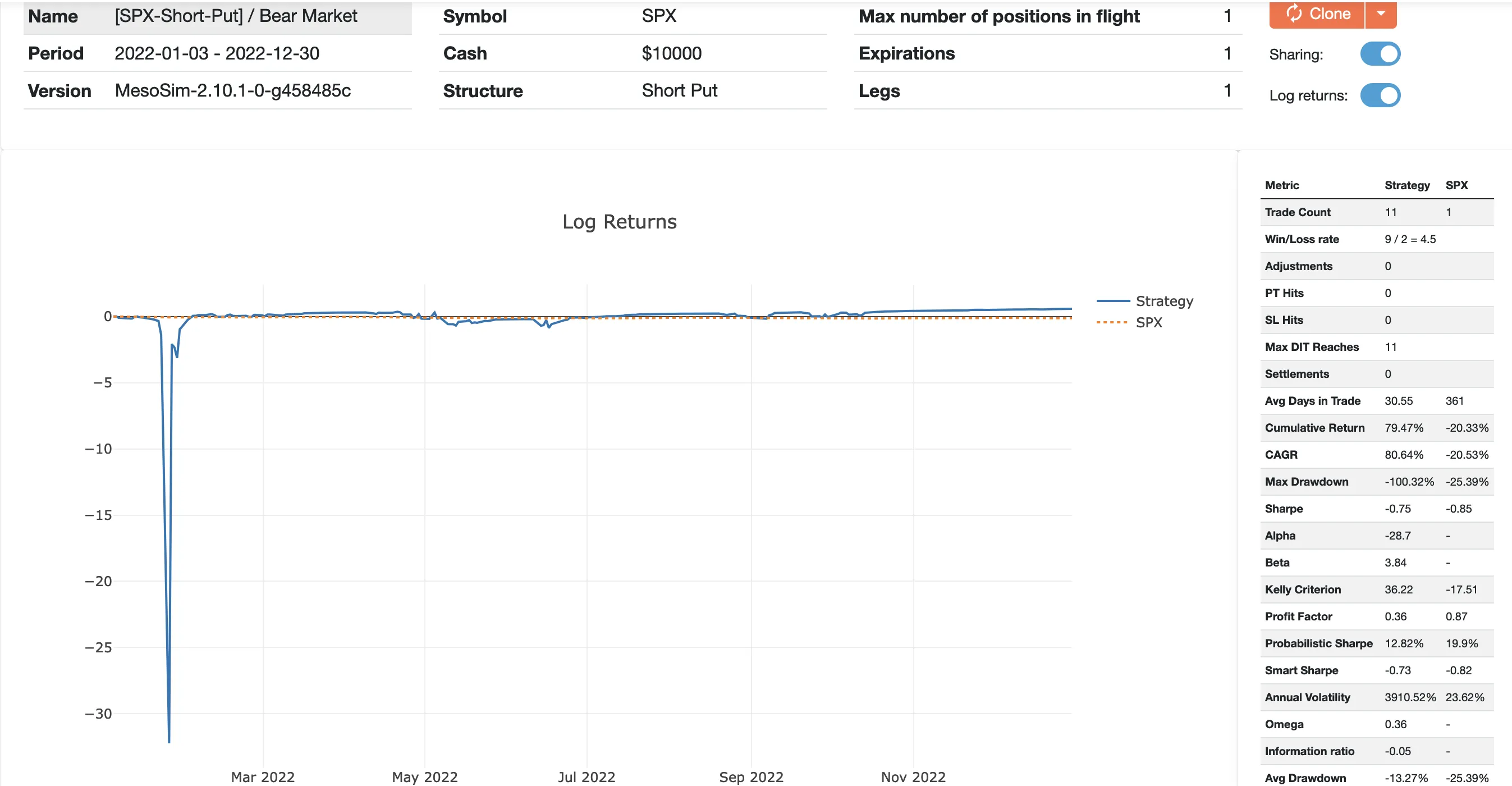
This simple strategy can be highly profitable in bull markets, but it can result in significant losses
during bear markets and sudden down moves.
MesoSim was created to study options trading strategies. It offers numerous built-in templates demonstrating key features as well as ready-to-use strategies.
For simulating Option Writing, we will utilize the [SPX-ShortPut] built-in template.
The above screenshots capture the overview of two runs for different time periods:
Trailing Stops are well known to equity, futures and options traders alike. The idea is simple: As the profit increases we store the highest profit achieved (high watermark) and create a stop order relative to the high watermark. This way, our stop loss will not be fixed, but it will continuously move higher as the strategy gains.
Programatically it can be described as:
At entry:
Set pnl_high_watermark to 0.
Whencurrent_pnl > pnl_high_watermark:
Set pnl_high_watermark to current_pnl.
Whencurrent_pnl < pnl_high_watermark * x%:
Exit the position.
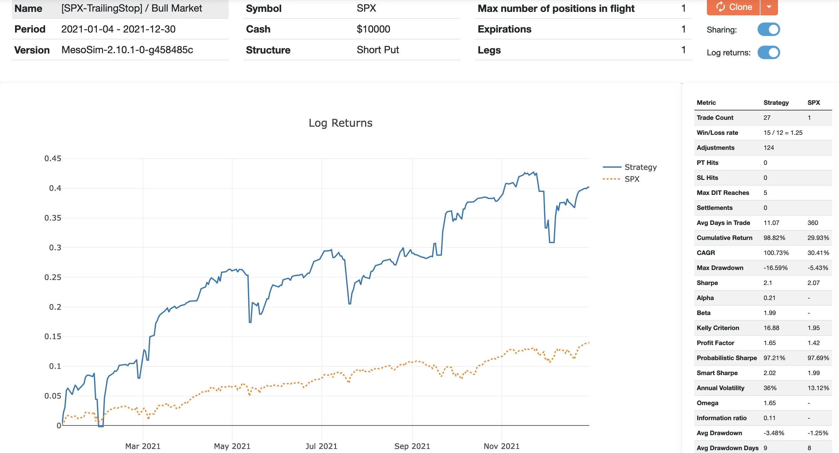
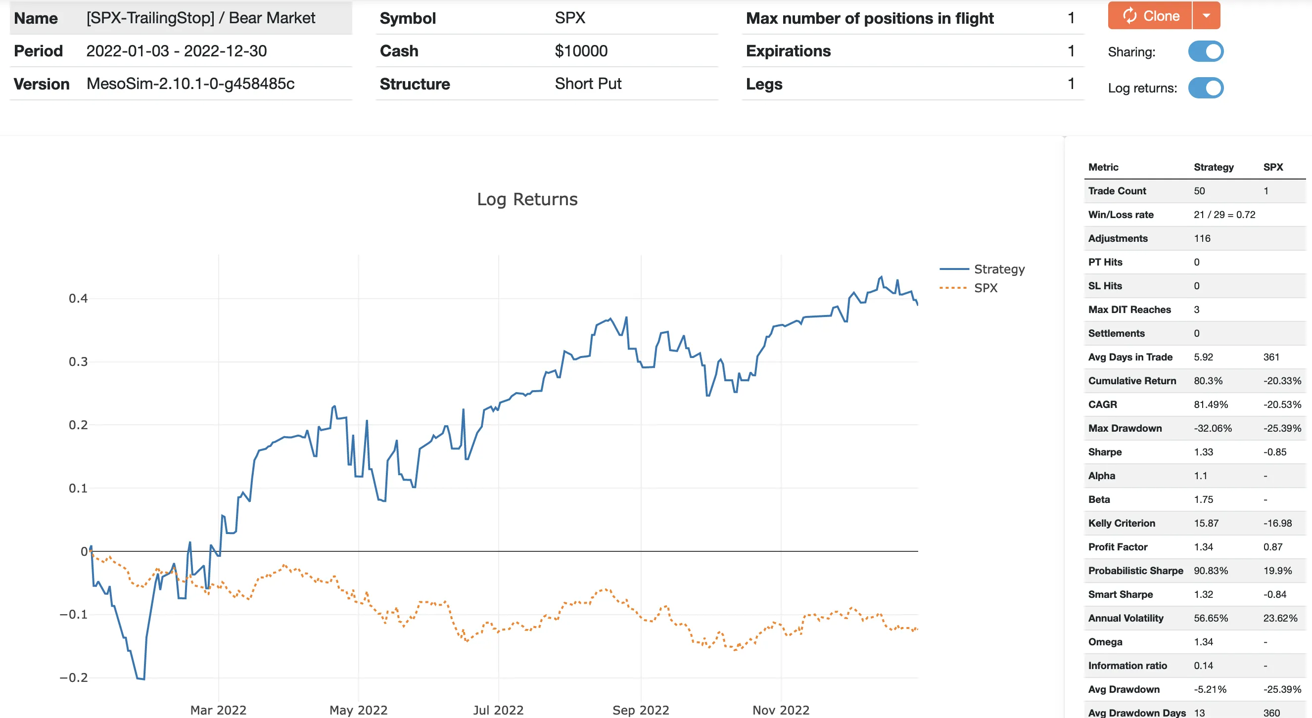
To explore how a trailing stop could enhance a trading strategy - such as option writing- in different market conditions, we will implement it in MesoSim. The above logic can be translated into a Strategy Definition as follows:
At entry initialize pnl_high_watermark variable to 0:
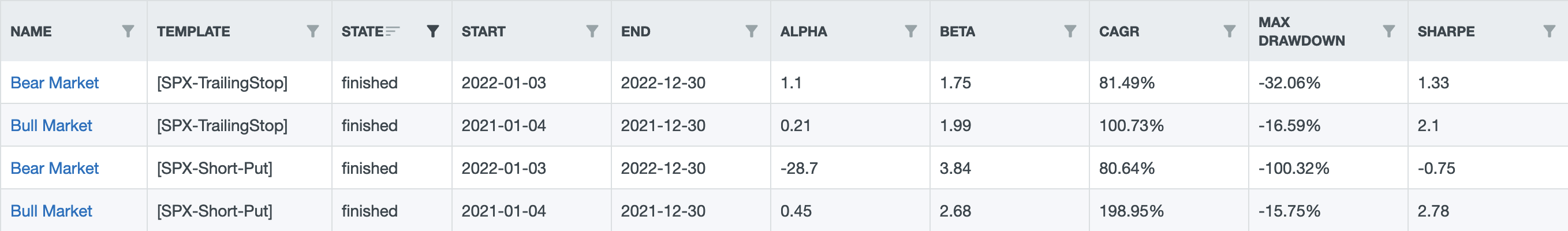
When comparing the original Short Put runs with the Trailing Stop version, we can conclude that the trailing stop signifficantly improved the strategy performance in Bear market. In contrast, the results in bull market became more modest, although it remains fairly good (with a sharpe ratio around 2).
Trailing stop is a dynamic approach to increase strategy performance. It has proven to be beneficial for the simple SPX Put Writing strategy by locking in gains without sacrificing much upside potential.
Someone interested in this approach should try different relative ranges from the high watermark to see how it affects her strategy performance.
MesoSim v3 Migration Note
This article was originally written for MesoSim v2. The examples and terminology have been updated to match the MesoSim v3 Strategy Definition format. For details, see the MesoSim v3.0 release announcement and the v2→v3 migration guide. The performance metrics, described behavior, and referenced run results reflect the original v2 behavior. If you rerun the referenced strategies on MesoSim v3, results may differ slightly due to behavioral changes in the simulator.
John Locke (@Locke4Success) is a reputable source when it comes to Options Trading Strategies. You can find many of his trading strategies on YouTube, for free.
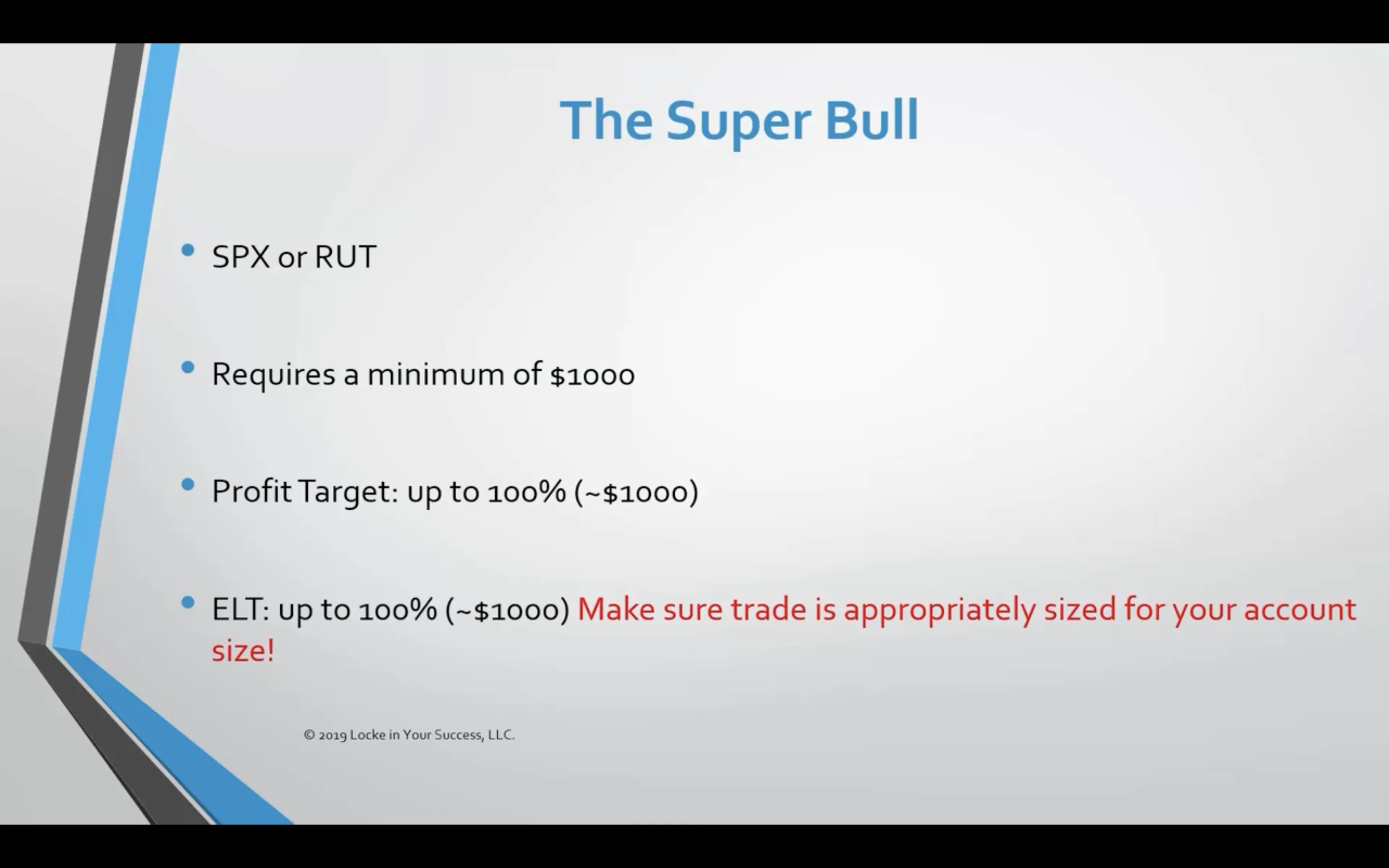
His strategies and their variants are often simulated with MesoSim.We are now adding his Super Bull strategy as a featured trade to our strategy library.
The rules were constructed as discussed in his youtube videos.
The strikes are selected in a manner where the long legs are positioned 20 points above the current price of the underlying asset and the shorts are chosen to achieve a Risk/Reward ratio that is close to 1.0
The strike closest to 20 points above the underlying price can be determined by setting the Complex StrikeSelector’s Target to underlying_price + 20 and specifying the constraint to ensure that the chosen leg’s strike will be always above the underlying price. This constraint is necessary because the Selector selects the nearest contract to our target, which - in some cases - may be below the underlying price.
The Statement field of the selector is evaluated for each contract and represents the strike. According to the SuperBull rules, our target will be 20 points above the current underlying price.
While John suggests aiming for a 1:1 Risk/Reward ratio, he shows multiple examples where the trade is initiated with a ratio lower than that. He explains that this is due to the unusual volatility skew observed on those particular days. In such trades, the risk/reward ratio was around 1.5 at the initiation.
John suggests that the trade should be sized so that it risks a maximum of 10% of the account size. This rule was implemented in our run using Entry.AbortConditions: We abort the entry if the Entry Debit would be greater than 10% of our NAV.
In our initial attempts, we used one contract for each leg. This turned out to be inadequate: Most of the time we under-sized the position (Maximum Risk was around 1% of NAV). To alleviate this problem we introduced Entry.QtyMultiplier to MesoSim, which is capable of scaling all the legs, once they are identified. We leverage this feature to target a maximum loss of 10% (in terms of account size) for our trades.
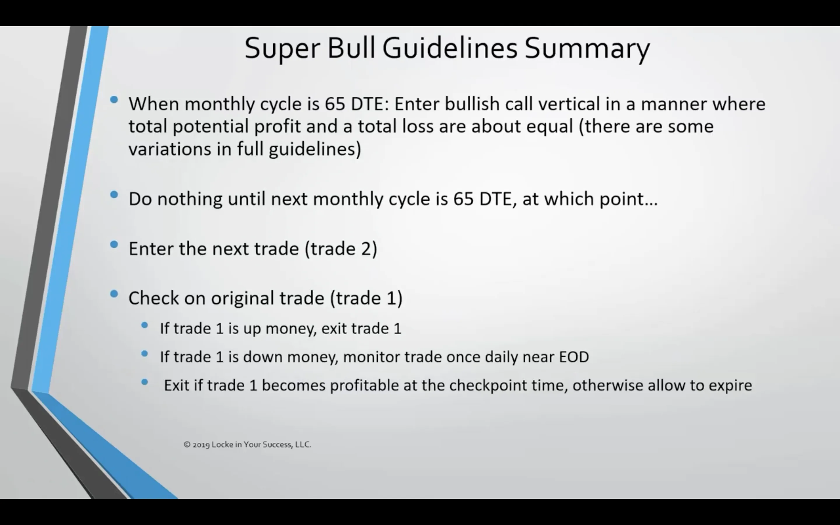
The exit rules for the strategy can be summarized as follows:
When the next monthly expiration becomes 65 days away, we enter a second trade. From that point onwards, we monitor the progress of the first trade. If the first generates a positive return, we exit the trade. However, if the first trade is at a loss we wait until it becomes profitable or reaches expiration.
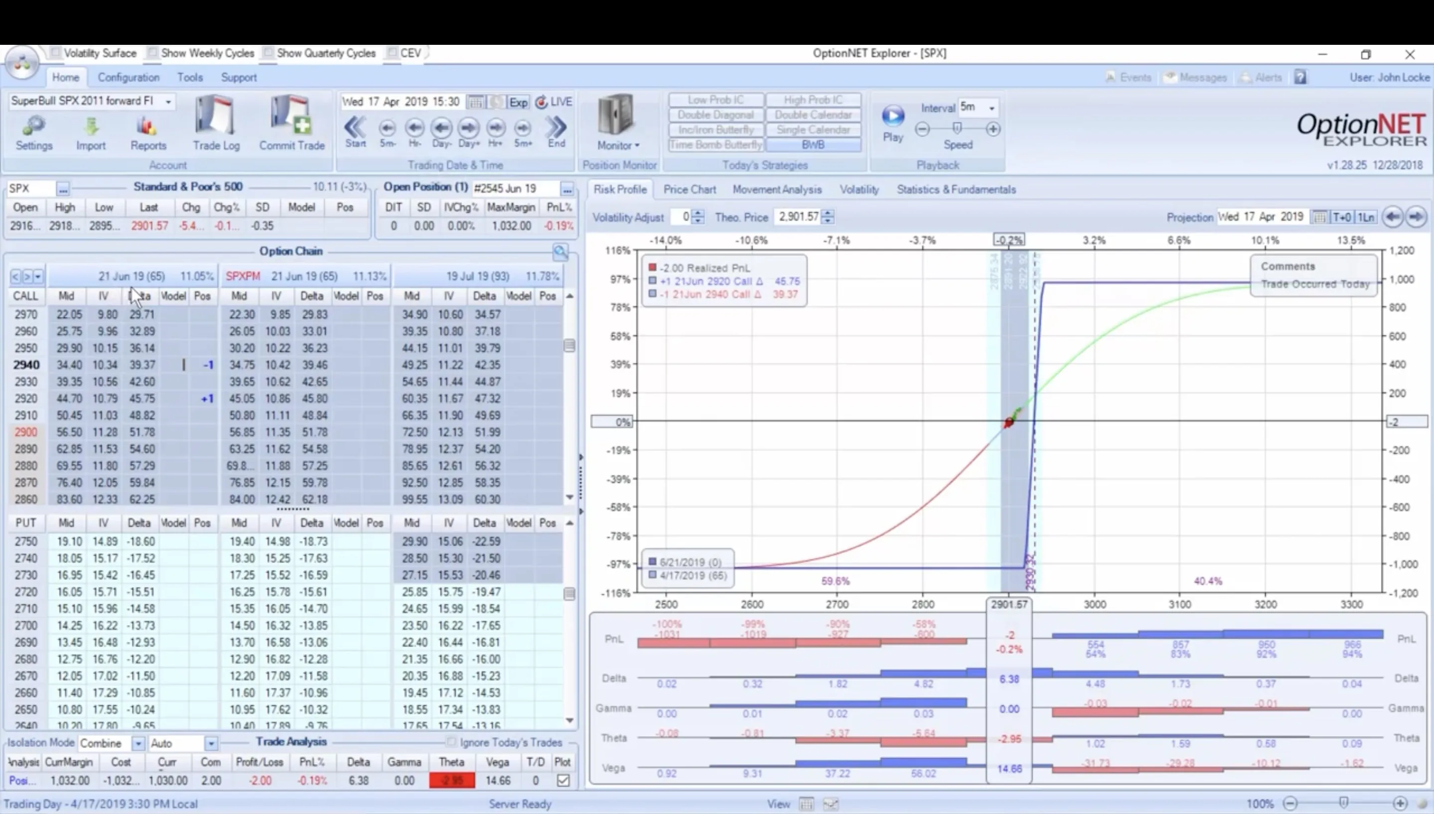
OptionNet Explorer is frequently utilized by options traders for modeling and manually simulating trades. It is essential to comprehend the accuracy and limitations of its simulation and real trading accuracy before engaging in trading activities. This section provides concise insights into these limitations, allowing the reader to better understand the comparison between MesoSim and OptionNet simulated results.
OptionNet Explorer can be utilized for initiating and monitoring live trades. However, there is one potential accuracy issue to be aware of. When entering complex (multi-legged) trades using the compounded Option Price, the individual leg prices in OptionNet often differ from the actual fills. Therefore, it is necessary to manually adjust the prices of the individual legs after entering the trade. This adjustment can be performed using the Trade Log window.
In contrast, MesoSim’s performance reporting tracks daily NAV values and computes quantitative performance metrics for both the strategy and the benchmark, such as Sharpe, Sortino, Omega, and more.
This information provides a more precise representation of the strategy’s performance, allowing the user to better understand its expected performance.
info
Please note that we do not mean to suggest that MesoSim is better than OptionNet. Instead, we state that OptionNet's functionality can be extended by MesoSim's automated backtesting and performance reporting capabilities.
In other words: MesoSim is a companion service to OptionNet Explorer.
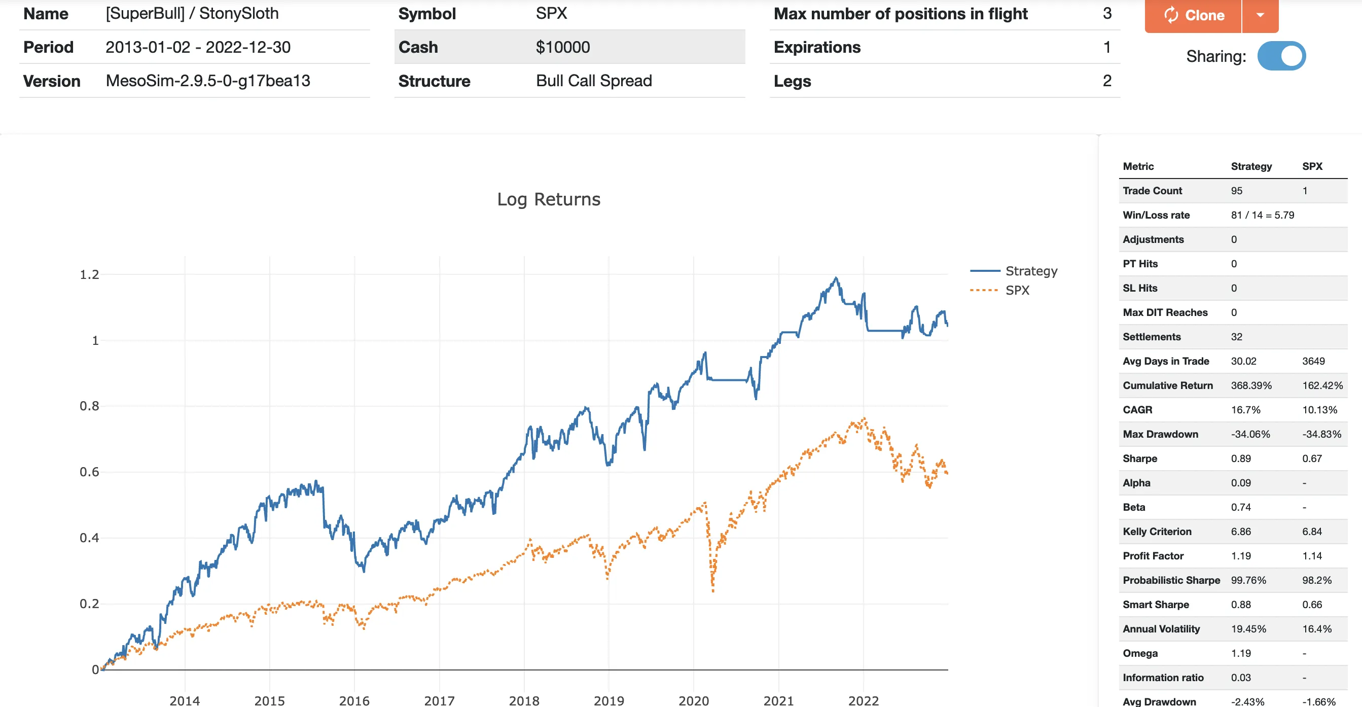
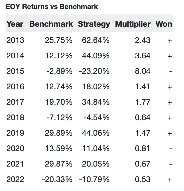
Our win rate of 85.2% (81/95) confirms that we are close to what John achieves (86%) with this trade.
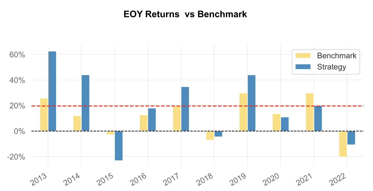
Both the Log Return and yearly breakdown charts show that the trade performs well during Bull Markets, such as 2013-2014, 2019, and 2021. However, it exhibits higher volatility during sideways markets.
If we compare SuperBull with the S&P-500 Buy and Hold strategy we can conclude that it performs better in the validation period:
Higher CAGR: 16.7% vs 10.11%
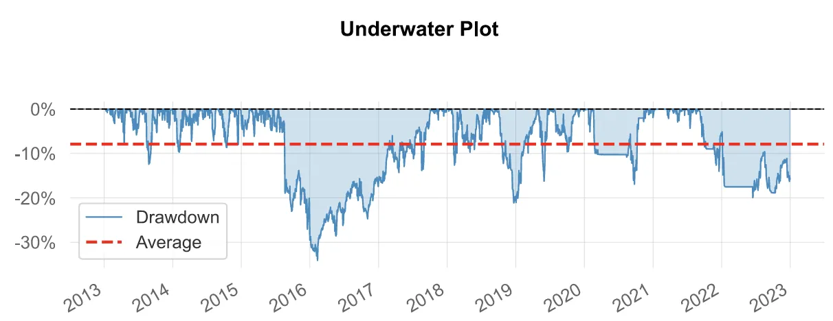
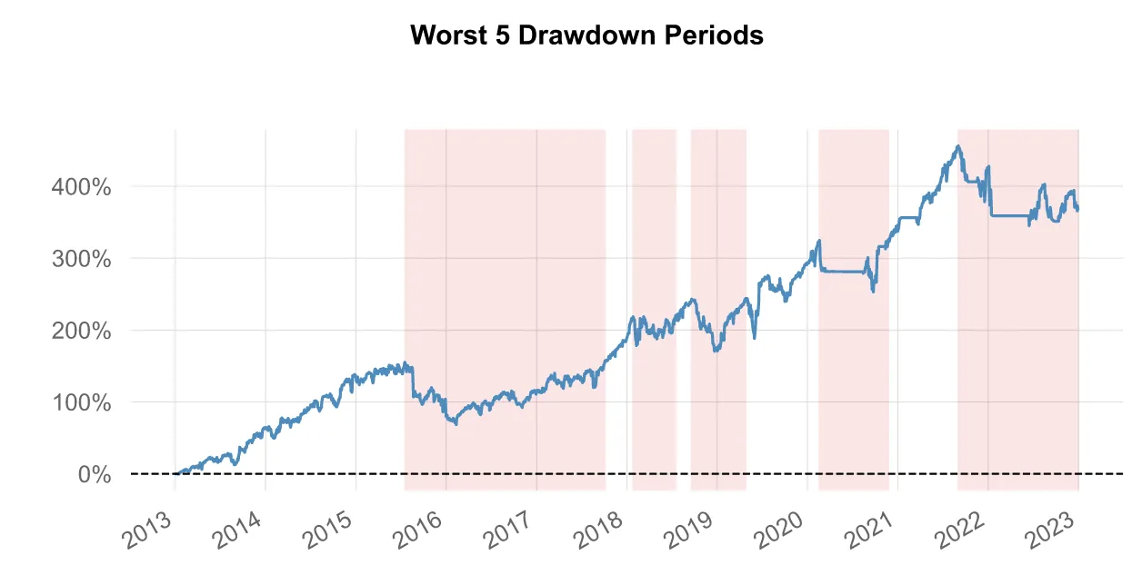
Slightly lower max drawdown: -34.06% vs -34.83%
Improved Sharpe ratio 0.89 vs 0.67
It has low margin requirements
Surprisingly, this strategy didn't exhibit a large drawdown during COVID as the Maximum Loss based Entry Filter prevented it from entering during market turmoil.
Rafael Munhoz, a key contributor to our community has thoroughly analyzed this trade and developed his own variant. Based on his experience, it proved challenging to find optimal trades that offered a 1:1 risk/reward ratio. He made adjustments to the trade to address these challenges and generously shared his results with us.
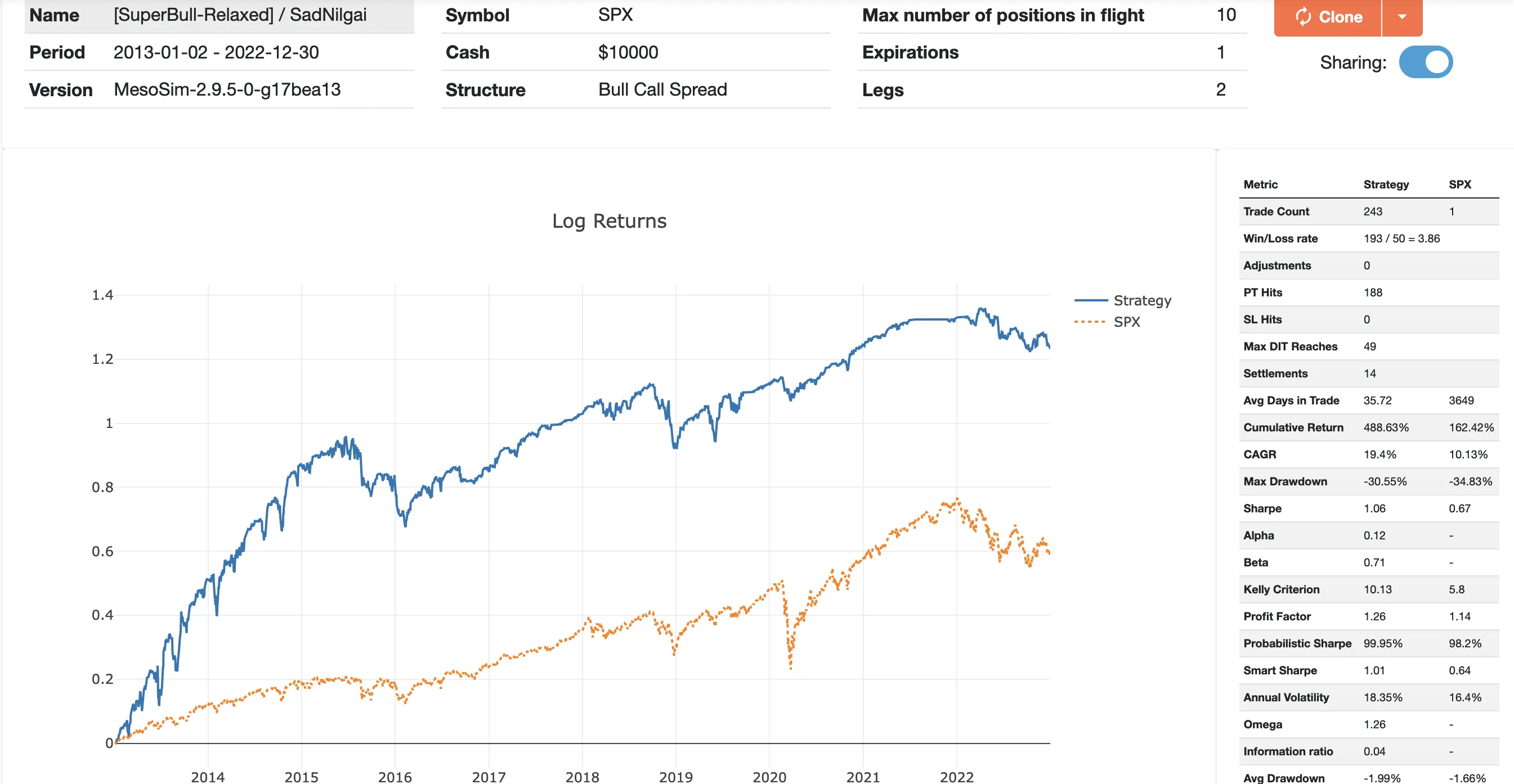
His results are improving the original trade by having higher CAGR, reduced Drawdown, (and therefore) improved Sharpe:
CAGR: 19.4% vs 16.7%
Max Drawdown: 30.55% vs 34.06%
Sharpe: 1.06 vs 0.89
Similar to the original trade, the Relaxed SuperBull also excels in bull markets andit has outstanding performance in the 2013-2014 period.
Due to its more dynamic exit criteria and re-entry rules, it responds fairly well to crashes, such as COVID.
However, unlike the other trade, this variant demands more attention from the trader as the entries and exits are more frequent and dynamic compared to the original strategy.
Both Rafael and ourselves believe that John's trade is worth studying. None of us is affiliated with John in any way.
We would like to thank John Locke and Rafael Munhoz for sharing the SuperBull and the SuperBull-Relaxed trades with the options trading community!
MesoSim v3 Migration Note
This article was originally written for MesoSim v2. The examples and terminology have been updated to match the MesoSim v3 Strategy Definition format. For details, see the MesoSim v3.0 release announcement and the v2→v3 migration guide. The performance metrics, described behavior, and referenced run results reflect the original v2 behavior. If you rerun the referenced strategies on MesoSim v3, results may differ slightly due to behavioral changes in the simulator.